FEniCS example - Kirsch’s problem¶

The problem¶

We will solve Kirsch’s probelm for a plate with dimensions $L_X \times L_y$ having a circular hole with a radius of $a$

We can solve a quarter problem due to symmetry but for this demonstration we will solve the entire domain.

As stated in the installation guide we rely heavily on Numerical tours of Computational Mechanics using FEniCS. A more comprehensive tutorial, dealing with various other topics as well, can be found in the FEniCS website

We will consider the following dimensions and constants:

\[\begin{split} L_X = L_y = 2 \\ \\ r=0.25 \\ \\ E=200e3 \ \ \text{Young's modulus}\\ \\ \nu = 0.32 \ \ \text{Poisson ratio}\\ \\ \sigma_{\inf} = 0.1 \ \ \text{the applied traction} \end{split}\]

Remeber we are solving a linear elastic problem here. As such, the constitutive relation we use is the one discussed in the section on elasticity.

To solve our problem we need to define it’s variational form (we will make use of the virtual work principle you learnet a few years ago).

In other words we are trying to find the displacements $\mathbf{u}$ which is an element in a function space $\textbf{V}$ such that : $$ \mathbf{\int_{\Omega} \sigma \left( u \right) : \epsilon(v) d\Omega = \int_{\Omega} \delta u(\sigma_{\inf} \cdot n) d \Omega} $$

With $\Omega$ being the entire domain, and $\mathbf{v}$ being an element of the same space function as $\mathbf{u}$.

Mesh generation¶

It is possible to convert meshes from varisou formats to an xml format which FEniCS can read, however for simplicity we will using mshr which can be installed using : “conda install -c conda-forge mshr”

Imports¶

We will need to import the dolfin interface to FEniCS. Similarly we will import mshr for generating the mesh.

from dolfin import *
from mshr import *
import matplotlib.pyplot as plt #we import matplotlib for plotting 
import numpy as np
#from vedo.dolfin import *
plt.style.use('ggplot')

Define the problem domain¶

Lx = 1. #Half the size of the plate in x
Ly = 1. #Half the size of the plate in y
r = 0.5 # hole radius
N= 50 #mesh density
# use a boolean substraction between the plate and a circle to generate a hole
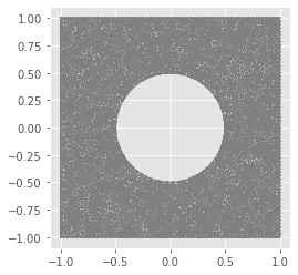
domain= Rectangle(Point(-Lx,-Ly), Point(Lx, Ly)) - Circle(Point(0., 0.), r) 
#declare the domain and mesh density
mesh = generate_mesh(domain, N)
#plot the mesh
dolfin.plot(mesh)
plt.show()

png

Alternative: we dont need a very fine mesh far from the hole so: ADD mesh from gmsh

Next we define the surfaces of importance

tol = 1e-14
class Tractions(SubDomain):
    def inside(self, x, on_boundary):
        return near(x[1], Ly) and on_boundary
class SymY(SubDomain):
    def inside(self, x, on_boundary):
        return near(x[1], -Ly) and on_boundary
class SymX(SubDomain):
    def inside(self, x, on_boundary):
        return near(x[0], 0) and on_boundary

# find exterior
facets = MeshFunction("size_t", mesh, 1)
facets.set_all(0)
Tractions().mark(facets, 1)
SymY().mark(facets, 2)
#SymX().mark(facets, 3)
ds = Measure('ds', subdomain_data=facets)

Next, we will want to define the:

elastic constants
load
are we in plane strain or plane stress (why?)
the strain operator
our constitutive relation (stress as a function of strain)

#Define our constants 
E = Constant(200e3)
ni = Constant(0.32)
G = E/(2.*(1.+ni))
lambdaPE = E*ni/(1+ni)/(1-2*ni) # plane strain
lambdaPS = ni*E/(1-ni*ni) # plane stress
twoDstate = "p.strain"

#load
SigmaInf = 1000


def eps(v):
    return sym(grad(v))

def sigma(v):
    lamda = lambdaPE
    if twoDstate == "p.stress":
        lamda = lambdaPS
    return lamda*tr(eps(v))*Identity(2) + 2.0*G*eps(v)

We will solve our problem using a continous lagranage polynoms (2$^{nd}$ degree)

#The function space: 
V = VectorFunctionSpace(mesh, 'Lagrange', degree=2)

#The variational form of our probelm:
du = TrialFunction(V)
u_ = TestFunction(V)
u = Function(V, name='Displacement')
a = inner(sigma(du), eps(u_))*dx

#Apply tractions on the top and bottom 
T = Constant((0, SigmaInf))
L = dot(T,u_)*ds(1) -dot(T,u_)*ds(2)

# The symmetry boundary consition:
#SymBC = [DirichletBC(V.sub(0), Constant(0.), facets, 3)]
#      DirichletBC(V.sub(1), Constant(0.), facets, 2)]
#SymBC =[  DirichletBC(V.sub(1), Constant(0.), facets, 2)]
#solve
solve(a == L, u)

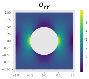
p = plot(sigma(u)[1, 1]/T[1], mode='color')
plt.colorbar(p)
plt.title(r"$\sigma_{yy}$",fontsize=26)
plt.show()

png

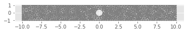
if you wish to automate the process, or at least parts of it, you can easily define a function and loop over the plate’s dimensions.

Below is an example for a function which gets as inputs the values of $L_x,L_y,r,N$ and returns a meshed geometry.

You can follow this example to extract the maximum value of $\sigma_{yy}$ as a function of $L_x / r$ and $L_y/r$ to examine the validity of the asymptotic solution.

def Kirsch(Lx,Ly,r,N):
    #r = 0.5 # hole radius
    #N= 50 #mesh density
    # use a boolean substraction between the plate and a circle to generate a hole
    domain= Rectangle(Point(-Lx,-Ly), Point(Lx, Ly)) - Circle(Point(0., 0.), r) 
    #declare the domain and mesh density
    mesh = generate_mesh(domain, N)
    #plot the mesh
    dolfin.plot(mesh)
    plt.show()
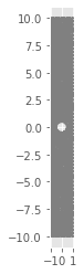
r,N=0.5,50

Kirsch(10,1,r,N)

png

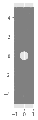
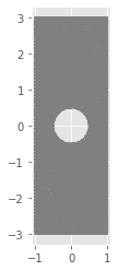
LxVec=[10,5,3]
for Lx in LxVec:
    Kirsch(Ly,Lx,r,N)

png

FM036004-Notes

FEniCS example - Kirsch’s problem¶

The problem¶

Mesh generation¶

Imports¶

Define the problem domain¶