J controlled fracture#
HRR#
Note
The HRR fields were published in 1968 by (J.R. Rice and G.F> Rosengren)[https://doi.org/10.1016/0022-5096(68)90013-6] and by (J.W. Hutchinson)[https://doi.org/10.1016/0022-5096(68)90014-8]
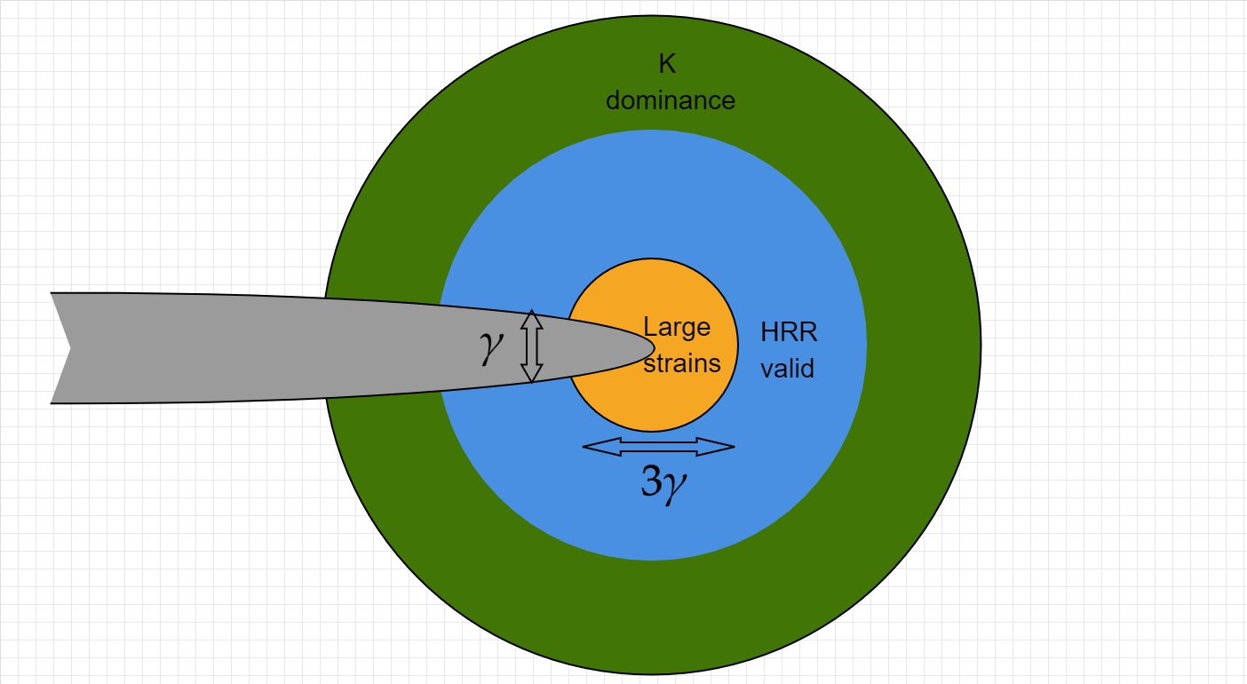
The HRR field, named after Hutchinson Rice and Rosengren is the solution for the mechanical fields at the tip of a stationary crack in a power law material.
The load is assumed to increase monotonically, thus allowing the use of the deformation theory of plasticity. As we mentioned previously, the deformation theory theory can be thought of as non-linear elasticity with the relation.
Writing down the \(J\) integral for \(r \to 0\) :
We can estimate that the integrand have the form of \(\frac{f(\theta)}{r}\)
This implies that
if we expand \(\sigma_{ij}\) into a series around \(r \to 0\) such that
we can obtain for \(r \to 0\) where the plastic strains are much greater than the elastic ones:
Since we required earlier that \(\sigma \cdot \epsilon \propto r^{-1}\) it implies that \(s+sn=-1\) and thus \(s\) which will lead to the strongest singularity is
Now, the HRR stress and strain fields (for \(r \to 0\)) are given by:
Note
For \(n \to 1\) we obtain a \(r^{-1/2}\) singularity
Using the HRR fields in the \(J\) integral will lead to
With \(k_n\) being:
and finally
It is time to find the angular dependency of the stress and strain (but we wont)
To do so, one need to introduce a stress function \(\phi\) whose derivatives define \(\sigma\).
Crack growth resistance curves#
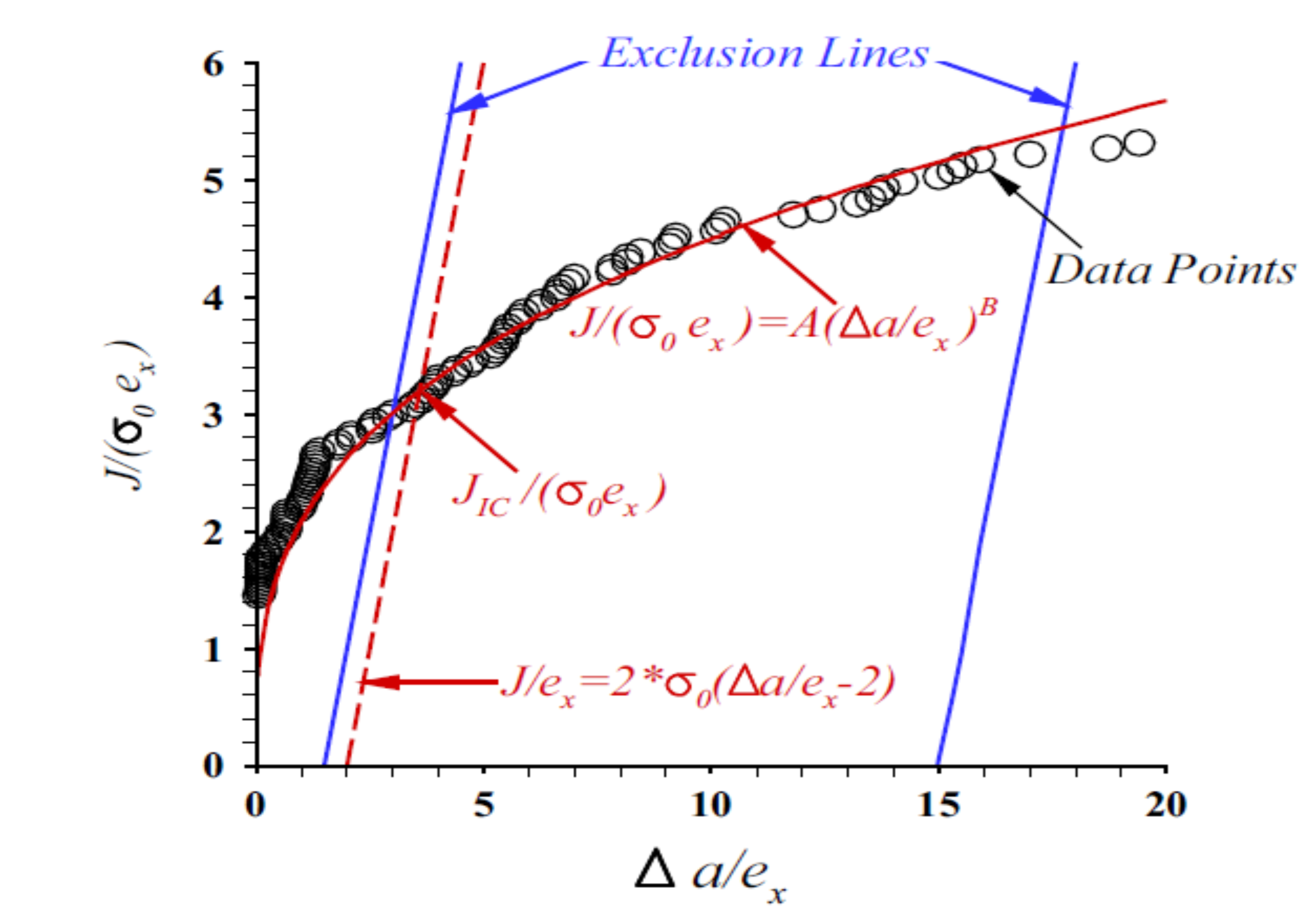
The value of the tearing modulus is calculated by applying:
on the polynomial fit to the data points between the exclusion lines.
Similar to the way we handeled \(G\) we can examine the stability of a growing crack by comparing the driving force for crack growth as :
with \(\color{red}{\Delta}\) being the applied displacement and \(\color{blue}{C_m,P}\) being the machine compliance and applied load.
We can easily obtain
When the machine is infinitely stiff (\(\color{blue}{C_m} \to \infty\) - load control) we are left with
A crack will grow in a stable manner when \(J=J_R\) and \(T_{app} \leq T_R\)
A crack will grow in an unstable manner when \(J=J_R\) and \(T_{app} \gt T_R\)