Kirsch’s Infinite Plate¶

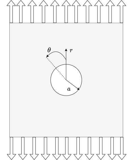
Consider a 2D plate containing a circular hole and being subjected to remote tensile load $\sigma_{\inf}$.

Taking under consideration the boundary conditions, we require our stress to be zero on the hole’s free surface:

\[ \sigma_r (r=a, \theta) = \tau_{r \theta} (r=a, \theta)=0 \]

We will start by considering a circular portion of the plate concentric with the hole and having a radius large enough with resect to a. The stresses will effectively be the same as in the plate without the hole and thus:

\[\begin{split} \begin{align*} & \sigma_r =\sigma_{\inf} cos^2 \theta = \sigma_{\inf} \frac{1}{2} (1+cos2\theta) \\ \\ & \tau_{r \theta} = -\sigma_{\inf} \frac{sin 2\theta}{2} \\ \end{align*} \end{split}\]

The stress distribution in the plate can be regarded as having two parts, the first arising from the normal applied traction and is $\frac{\sigma_{\inf}}{2}$ and the second part having an angular dependence.

A good guess for $\Phi$, seems to have the general form :

\[ \Phi = g(r) + f(r)cos2\theta \]

Let us ignore $g(r)$ for now.

Substituting $\Phi$ into the bi-harmonic equation we readily obtain:

\[ \left ( \frac{d^2}{dr^2} + \frac{1}{r}\frac{d}{dr} - \frac{4}{r^2} \right )\left ( \frac{d^2 f}{dr^2} + \frac{1}{r}\frac{df}{dr} - \frac{4f}{r^2} \right ) = 0 \]

A general solution to this ODE on $f(r)$ will have the form :

\[ f(r) = Ar^2 + Br^4 + \frac{C}{r^2} + D \]

and so the stress components are

\[\begin{split} \begin {align*} & \sigma_{rr} = \frac{1}{r^2} \frac{\partial^2 \Phi}{\partial \theta ^2} + \frac{1}{r}\frac{\partial \Phi}{\partial r} = -\left( 2A +\frac{6C}{r^4} + \frac{4D}{r^2}\right)cos 2 \theta\\ \\ \\ & \tau_{r \theta} = \frac{1}{r^2} \frac{\partial^2 \Phi}{\partial \theta \partial r} + \frac{1}{r^2}\frac{\partial \Phi}{\partial \theta} = \left( 2A + 6Br^2 - \frac{6C}{r^4} - \frac{2D}{r^2}\right)sin 2 \theta \\ \\ & \sigma_{\theta \theta} = \frac{\partial ^2 \Phi}{\partial r^2} = \left( 2A + 12Br^2 + \frac{6C}{r^4}\right)cos 2 \theta \end{align*} \end{split}\]

From the conditions prescribed above we obtain:

\[ A= - \frac{1}{4} \sigma_{\inf} \quad ; \quad B=0 \quad ; \quad C=-\frac{a^4}{4}\sigma_{\inf} \quad ; \quad D=\frac{a^2}{2}\sigma_{\inf} \]

The uniform tension $\frac{1}{2}\sigma_{\inf}$ is accounted for by $g(r)$ which can be written as :

\[ g(r) = A_1log (r) + B_1r^2log(r) +C_1r^2 + D_1 \]

which is a general solution for a stress distribution symmetrical about an axis1.

Adding the two parts of the solution we finally obtain:

\[\begin{split} \begin{align*} \sigma_{rr} &= \frac{\sigma_{\inf}}{2} \left( 1 - \frac{a^2}{r^2}\right) + \frac{\sigma_{\inf}}{2} \left( 1 + \frac{3a^4}{r^4} - \frac{4a^2}{r^2}\right)cos2\theta \\ \\ \sigma_{r\theta} &= -\frac{\sigma_{\inf}}{2} \left( 1 - \frac{3a^4}{r^4} + \frac{2a^2}{r^2}\right) sin2\theta\\ \\ \sigma_{\theta \theta} &= \frac{\sigma_{\inf}}{2} \left( 1 + \frac{a^2}{r^2}\right) - \frac{\sigma_{\inf}}{2} \left( 1 + \frac{3a^4}{r^4}\right)cos2\theta \\ \end{align*} \end{split}\]

For $r=a$ we can see that $$ \sigma_{rr}=\tau_{r \theta} =0 \quad ; \quad \sigma_{\theta \theta} = \sigma_{\inf} \left(1-2cos2\theta \right) $$

the maximum stress experienced appear at $\theta = \pi /2 ; 3\pi/2$ where $\sigma_{\theta \theta} = 3\sigma_{inf}$

Note that for $\theta=0,\pi$ we obtain $\sigma_{\theta \theta}=-\sigma_{\inf}$.

From the figure below, it is evident that the stress magnitude rapidly decreases to the remote load as $r$ increases.

1: Theory of Elasticity; J.N. Goodier & S. Timoshenko 1951, New York.

FM036004-Notes

Kirsch’s Infinite Plate¶