Elasticity - A Reminder¶

Assuming everyone has taken ME035043, we will simply recap on some basic concepts. In case you need a more in-depth reminder, I recommend Applied Mechanics of solids by A.F. Bower and Elasticity: theory and applications by A.S. Saada Consider the following not as a lecture notes but more as a quiz for yourslef. If you are not familiar with any of the terms or equations - you need to go to the recommended sources.

Strain¶

Given a displacemnts vector \(u\) the infinitsimal strain is defined as :

\[ { \epsilon_{ij} = \frac{1}{2} \left( \frac{\partial{u_j}}{\partial{x_i}} + \frac{\partial{u_i}}{\partial{x_j}} \right ) \quad ; \quad \pmb{\epsilon} = \frac{1}{2} \left( \pmb{u} \nabla + (\pmb{u} \nabla)^T \right )} \]

\[\begin{split} \epsilon_{ij} = \Large {\begin{bmatrix} \frac{\partial{u_1}}{\partial{x_1}}& \frac{1}{2} \left( \frac{\partial{u_1}}{\partial{x_2}} + \frac{\partial{u_2}}{\partial{x_1}} \right ) & \frac{1}{2} \left( \frac{\partial{u_1}}{\partial{x_3}} + \frac{\partial{u_3}}{\partial{x_1}} \right ) \\ \frac{1}{2} \left( \frac{\partial{u_2}}{\partial{x_1}} + \frac{\partial{u_1}}{\partial{x_2}} \right )& \frac{\partial{u_2}}{\partial{x_2}} & \frac{1}{2} \left( \frac{\partial{u_2}}{\partial{x_3}} + \frac{\partial{u_3}}{\partial{x_2}} \right ) \\ \frac{1}{2} \left( \frac{\partial{u_3}}{\partial{x_1}} + \frac{\partial{u_1}}{\partial{x_3}} \right )& \frac{1}{2} \left( \frac{\partial{u_3}}{\partial{x_2}} + \frac{\partial{u_2}}{\partial{x_3}} \right ) & \frac{\partial{u_3}}{\partial{x_3}} \\ \end{bmatrix} } \end{split}\]

Note

In many FE codes the shear strains output is given as “Engineering shear strain” such that

\[ \gamma_{ij}=2\epsilon_{ij} \quad for \quad i\ne j \]

The strain tensor can be divided to deviatric \(\pmb(e)\) and volumetric \(\epsilon_{kk}\) parts such that

\[ J \approx 1+ \epsilon_{kk} \quad \text{\&} \quad \pmb{e} = \pmb{\epsilon} - \frac{1}{3}\pmb{I}\text{trace}(\pmb{\epsilon}) \]

The eigenvalues of \(\pmb{\epsilon}\) and corresponding eigenvectors will define the principal values \((e_i)\) and directions \((\pmb{n}^i)\) of the strain tensor.

Rotations¶

Stress¶

For (isotropic) linear elasticity, we can correlate the strains with the stresses using :

\[ \sigma_{ij} = \frac{E}{1+\nu}\left[ \epsilon_{ij} + \frac{\nu}{1-2\nu}\epsilon_{kk}\delta_{ij} \right] - \frac{E\alpha\Delta T}{1-2\nu}\delta_{ij} \]

or, fiven the stress tensor, we can obtain the strains following:

\[ \epsilon_{ij} = \frac{1+\nu}{E} \sigma_{ij} - \frac{\nu}{E}\sigma_{kk}\delta_{ij}+\alpha \Delta T\delta_{ij}\]

Here, \(E\) is Young’s modulus, \(\nu\) is Poisson’s ratio, \(\alpha\) the thermal expansion coefficient and \(\Delta T\) stands for temperature increase (decrease)

The shear modulus \(G\) is defined as :

\[ G=\frac{E}{2 (1+\nu)} \]

Strain Energy density¶

The strain energy density \([Joule/m^3]\) is defined as :

\[W = \int_{0}^{\epsilon} \sigma d\epsilon \]

Under linear elasticity we obtain

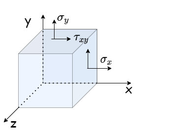
\[W_{elastic}=\frac{1}{2}E\epsilon^2 = \frac{\sigma^2}{2E}\]

Plane stress¶

Thin solids, (i.e. one dimension is significantly smaller than the other two) loaded in-plane, can be approximated using 2D plane stress assumptions. under this assumption :

\[ \sigma_{33} = \tau_{23} = \tau_{31} = \epsilon_{23} =\epsilon_{31} = 0\]

Plane strain¶

A solid body, whose deformation in one direction are severely restricted (consider the mid-sction of a thick body) can be assumed to be in a plane strain condition such that:

\[ \epsilon_{23}=\epsilon_{13}=\epsilon_{33}=0 \quad \& \quad \sigma_{33} \approx \nu \left( \sigma_{11} + \sigma_{22} \right) \]

Solution to elasticity problems (static)¶

Given an elastic body with applied tractions \(t_j^{ap}\) and displacements \(u_i^{ap}\) we seek to find a solution which will satisfy:

\[\begin{split} \begin{align*} & \epsilon_{ij} = \frac{1}{2} \left( \frac{\partial{u_j}}{\partial{x_i}} + \frac{\partial{u_i}}{\partial{x_j}} \right ) \\ & \sigma_{ij} = \frac{E}{1+\nu}\left[ \sigma_{ij} + \frac{\nu}{1-2\nu} \right] - \frac{E\alpha\Delta T}{1-2\nu}\delta_{ij} \\ & \frac{\partial \sigma_{ij}}{\partial x_i} + F_j =0 \quad (\text{equilibrium}) \end{align*} \end{split}\]

as well as the B.C:

\[ u_i = u_i^{ap} \quad \& \quad \sigma_{ij} n_j=t_i^{ap} \]

on the portions of the boundary where they are defined

FM036004-Notes