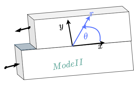
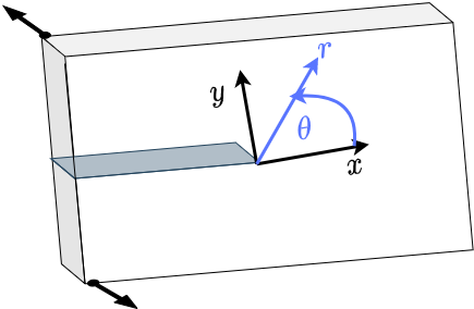
Stress Intensity Factors II

mode1

We will follow Williams’s approach[^I1]. The boundary conditions of our problem are such that the crack faces will be traction free:

\[ \sigma_{\theta \theta} = \sigma_{r \theta} = 0 \ \ ; \ \ (\text{for} \ \ \theta=\pm \pi ) \]

Next, remembering that the stresses in polar coordinate are expressed as : In polar coordinates, stresses are expressed as:

(6)\[\begin{split}\begin{align*} \sigma_{rr}& = \frac{1}{r^2} \frac{\partial^2 \Phi}{\partial \theta ^2} + \frac{1}{r}\frac{\partial \Phi}{\partial r}\\ \\ \tau_{r \theta}& = \frac{1}{r^2} \frac{\partial^2 \Phi}{\partial \theta \partial r} + \frac{1}{r^2}\frac{\partial \Phi}{\partial \theta} \\ \\ \sigma_{\theta \theta}& = \frac{\partial ^2 \Phi}{\partial r^2} \end{align*}\end{split}\]

The B.C leads to the requirement:

\begin{align*} &\phi_{,rr} = 0 &\left( \frac{1}{r}\phi_{,\theta}\right )_{,r} =0 \end{align*}

We know that \(\phi\) will depend on both \(r\) and \(\theta\). For the sake of having shorter equations, we can start be defining \(\psi\) such that:

\[ \nabla^2 \phi = \psi \]

and since we are looking for a solution for the bi-harmonic problem \(\nabla ^4 \phi =0\) we need to find \(\psi\) that will satisfy

(7)\[ \nabla ^2 \psi =0 \]

The following form will satisfy (7) :

(8)\[ \psi = r^{\lambda -1}f(\theta) \]

leading to

(9)\[ \nabla^2\psi = r^{\lambda -3}[f(\theta) (\lambda -1)^2+f^{''}(\theta)]=0 \]

Equation (9) is obviously satisfied for \(r=0\) and \(\lambda \geq 3\) otherwise, we must solve :

\[ (\lambda-1)^2f(\theta) +f^{''}(\theta) =0 \]

from which we can find that:

(10)\[ f(\theta) = A\sin(\lambda -1) \theta + B\cos(\lambda -1) \theta \]

plugging (10) into (7) & (8) leads to :

(11)\[ \nabla ^2 \psi =r^{\lambda -1}A\sin(\lambda -1) \theta + B\cos(\lambda -1) \theta \]

and finally \(\phi\) assumes the form:

(12)\[ \phi(r,\theta) = r^{\lambda+1}[\frac{A}{4 \lambda} \cos ((\lambda-1) \theta) + \frac{B}{4 \lambda} \sin ((\lambda-1) \theta) +C \cos ((\lambda+1) \theta) + D \sin ((\lambda+1) \theta)] \]

To find the coefficients in (12) we will first write explicitly the stresses.

To make our life easier (and to avoid stupid mistakes :) ) we will use the symbolic math python library sympy

#here we import the library
from sympy import *
init_printing(pretty_print=True, backcolor='Transparent',use_latex='png' ,fontsize='13pt', wrap_line=True,forecolor='Black')
---------------------------------------------------------------------------
ModuleNotFoundError                       Traceback (most recent call last)
/tmp/ipykernel_1762/2193309469.py in <module>
      1 #here we import the library
----> 2 from sympy import *
      3 init_printing(pretty_print=True, backcolor='Transparent',use_latex='png' ,fontsize='13pt', wrap_line=True,forecolor='Black')

ModuleNotFoundError: No module named 'sympy'

Next, we will define the symbols we are using:

phi, A,B,C,D = symbols('phi A B C D')
L, r, theta = symbols('lambda r theta',real=True)

Since we are about to calculate the stresses using (6) it will be usefull to define the operators used for those calculations:

def Srr(phi,r,theta):
  return (phi.diff(r)/r + (1/r**2)*phi.diff(theta,2))

def Srt(phi,r,theta):
  phi_t =(1/r)*phi.diff(theta)   
  return -phi_t.diff(r)


def Stt(phi,r,theta):
  return phi.diff(r,2)

Ok, almost good to go,

Next we need to define the function \(\phi\) based on (12) :

phi = r**(L+1) * ((A/4/L)*cos((L-1)*theta) + 
                  (B/4/L)*sin((L-1)*theta) + 
                  (C)    *cos((L+1)*theta) + 
                  (D)    *sin((L+1)*theta)  )
phi
../_images/SIF_Airy_9_0.png

Calculating the stresses is now a simple task:

sigma_rr = Srr(phi,r,theta)
sigma_rt = Srt(phi,r,theta)
sigma_tt = Stt(phi,r,theta)

And now \(\sigma_{rr}\) is given by:

temp = sigma_rr*4/r**(L-1)
temp =((A*apart(temp,A).coeff(A) + B*apart(temp,B).coeff(B)+C*apart(temp,C).coeff(C)+D*apart(temp,D).coeff(D)))
(r**(L-1)/4)*simplify(temp)
../_images/SIF_Airy_13_0.png

\(\sigma_{r\theta}\) by:

simplify(sigma_rt)
../_images/SIF_Airy_15_0.png

and \(\sigma_{\theta \theta}\)

simplify(sigma_tt)
../_images/SIF_Airy_17_0.png
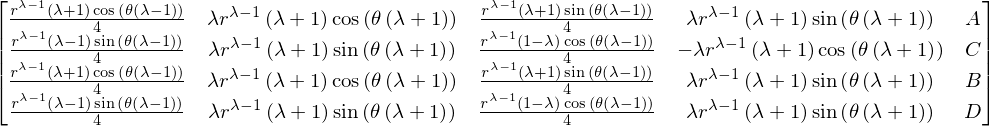
M = Matrix(([apart(sigma_tt,A).coeff(A), apart(sigma_tt,C).coeff(C), apart(sigma_tt,B).coeff(B), apart(sigma_tt,D).coeff(D),A],
           [apart(sigma_rt,A).coeff(A),apart(sigma_rt,C).coeff(C),  apart(sigma_rt,B).coeff(B), apart(sigma_rt,D).coeff(D),C],
           [apart(sigma_tt,A).coeff(A), apart(sigma_tt,C).coeff(C), apart(sigma_tt,B).coeff(B),apart(sigma_tt,D).coeff(D),B],
           [apart(sigma_rt,A).coeff(A), apart(sigma_rt,C).coeff(C), apart(sigma_rt,B).coeff(B),apart(sigma_tt,D).coeff(D),D]))
simplify(M)
../_images/SIF_Airy_18_0.png

The B.C, in conjuction with the stress expressions we have obtained can be written as a system of equations :

sigma_rtP = sigma_rt.subs(theta,pi)
sigma_rtN = sigma_rt.subs(theta,-pi)
sigma_ttP = sigma_tt.subs(theta,pi)
sigma_ttN = sigma_tt.subs(theta,-pi)

simplify_logic(sigma_ttN)
../_images/SIF_Airy_20_0.png

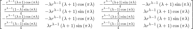
The solution we are looking for is of the form:

(13)\[\begin{split}\begin{bmatrix} M \end{bmatrix} \begin{bmatrix} A \\ B \\ C \\ D \end{bmatrix} =\begin{bmatrix} 0 \\ 0 \\ 0 \\ 0 \end{bmatrix}\end{split}\]
M = Matrix(([apart(sigma_ttP,A).coeff(A), apart(sigma_ttP,C).coeff(C),apart(sigma_ttP,B).coeff(B), apart(sigma_ttP,D).coeff(D)],
           [apart(sigma_rtP,A).coeff(A), apart(sigma_rtP,C).coeff(C),apart(sigma_rtP,B).coeff(B), apart(sigma_rtP,D).coeff(D)],
           [apart(sigma_ttN,A).coeff(A), apart(sigma_ttN,C).coeff(C),apart(sigma_ttN,B).coeff(B), apart(sigma_ttN,D).coeff(D)],
           [apart(sigma_rtN,A).coeff(A), apart(sigma_rtN,C).coeff(C),apart(sigma_rtN,B).coeff(B), apart(sigma_rtN,D).coeff(D)]))
simplify(M)
../_images/SIF_Airy_22_0.png

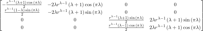
rearranging M such that :

M[0,:] = M[0,:]+M[2,:]

M[1,:] = M[1,:]+M[3,:]

M[2,:] = M[2,:]-M[0,:]

M[3,:] = M[3,:]-M[1,:]

We arrivae at:

Ma = M.copy()

Ma[0,:] = M[0,:]+M[2,:]

Ma[1,:] = M[1,:]-M[3,:]

Ma[2,:] = M[2,:]-M[0,:]

Ma[3,:] = M[3,:]+M[1,:]

simplify(Ma)
../_images/SIF_Airy_24_0.png
Ma.det()
../_images/SIF_Airy_25_0.png

for:

\[\lambda = \frac{n}{2} \ \ ; \ \ -\infty < n < \infty \]

the detreminant is always zero

We saw that the stress will behave as \(r^{\lambda -1}\) and the strain will follow the same power law.

This results in having the strain energy to be:

(14)\[\int\sigma\epsilon dA ~ \int r^{2 \lambda -2} dr d\theta ~r^{2 \lambda}\]

and for the energy to obtain a finite value we demand that \(2 \lambda >0\) leading to \( n \geq 1\)

LEt us now go row by row and look at the solutions for {A, B, C, D}

from the first row we obtain

\[C = -\frac{1}{4\lambda} A\]

for \(\lambda = 1,2,3....\infty\)

From the seond row we obtain

\[C = \frac{1-\lambda}{4\lambda (1+\lambda)} A\]

for \(\lambda = \frac{1}{2},\frac{3}{2},\frac{5}{2}....\infty\)

Similarly from the second bloc of M we obtain

\[D = -\frac{1}{4\lambda} B\]

for \(\lambda = \frac{1}{2},\frac{3}{2},\frac{5}{2}....\infty\)

and

\[D = \frac{1-\lambda}{4\lambda (1+\lambda)} B\]

for \(\lambda = 1,2,3....\infty\)

From the above solutions it is clear that we have two sets of solutions one for for \(\color{red}{\lambda = 1,2,3....\infty}\) for which

\[\begin{split} \color{red}{C = -\frac{1}{4\lambda} A \\ D = \frac{1-\lambda}{4\lambda (1+\lambda)} B } \end{split}\]

and one for \(\color{blue}{\lambda = \frac{1}{2},\frac{3}{2},\frac{5}{2}....\infty}\)

\[\begin{split} \color{blue}{C = \frac{1-\lambda}{4\lambda (1+\lambda)} A \\ D = -\frac{1}{4\lambda} B } \end{split}\]
mode3

We can write to final solution as a superposition of the two such that

\[\begin{split}\sigma_{rr} = \color{blue}{\sigma_{rr}^a}+ \color{red}{\sigma_{rr}^b }\\ \sigma_{r\theta} = \color{blue}{\sigma_{r \theta}^a}+ \color{red}{\sigma_{r \theta}^b }\\ \sigma_{\theta \theta} = \color{blue}{\sigma_{\theta \theta}^a}+ \color{red}{\sigma_{\theta \theta}^b}\end{split}\]

Looking for example at \(\sigma_{rr}\) it now reads (up to n=4) :

\[\begin{split} \sigma_{rr} = \color{blue}{\frac{r^{-1/2}}{4} \left( \frac{5}{2}\cos \frac{\theta}{2} - \frac{1}{2} \cos \frac{3 \theta}{2} \right ) A_0 ^a +\left( - \frac{5}{2}\sin \frac{\theta}{2} + \frac{3}{2} \sin \frac{3 \theta}{2} \right ) B_0^a } \\ + \color{red}{ \frac{1}{2} \left( 1+\cos 2 \theta \right)A_1 ^b } + \color{blue}{\frac{r^{1/2}}{4} \left( \frac{3}{2}\cos \frac{\theta}{2} + \frac{1}{2} \cos \frac{5 \theta}{2} \right )\\ A_1 ^a +\left( \frac{3}{2}\sin \frac{\theta}{2} + \frac{5}{2} \sin \frac{5 \theta}{2} \right ) B_1 ^a } \\ + \color{red}{ \frac{r}{4} \left(\cos \theta+ 3 \cos 3 \theta \right)A_2 ^b + \left( \sin \theta + \sin 3 \theta \right ) B_2 ^b} \end{split}\]

Restricting ourselves now to just one set of solutions such that \(\lambda = \frac{1}{2}\) we obtain:

\[\begin{split}\color{blue}{\sigma_{rr} = \frac{r^{-1/2}}{4} \left( \frac{5}{2}\cos \frac{\theta}{2} - \frac{1}{2} \cos \frac{3 \theta}{2} \right ) A_0 +\left( - \frac{5}{2}\sin \frac{\theta}{2} + \frac{3}{2} \sin \frac{3 \theta}{2} \right ) B_0 } \\ \color{blue}{\sigma_{r \theta} = \frac{r^{-1/2}}{4} \left( \frac{1}{2}\sin \frac{\theta}{2} + \frac{1}{2} \sin \frac{3 \theta}{2} \right ) A_0 +\left( + \frac{1}{2}\cos \frac{\theta}{2} + \frac{3}{2} \cos \frac{3 \theta}{2} \right ) B_0 } \\ \color{blue}{\sigma_{\theta \theta} = \frac{r^{-1/2}}{4} \left( \frac{3}{2}\cos \frac{\theta}{2} + \frac{1}{2} \cos \frac{3 \theta}{2} \right ) A_0 -\left( \frac{3}{2}\sin \frac{\theta}{2} + \frac{3}{2} \sin \frac{3 \theta}{2} \right ) B_0 } \\\end{split}\]

Finally

Substituting \(\theta = 0\) we obtain :

\(\sigma_{\theta \theta}(r,0) = \frac{A_0}{2 \sqrt(r)}=\frac{K_{I}}{\sqrt{2 \pi r}}\) which leads us to the immediate conclusion that \(A_0 = \sqrt{\frac{2}{\pi}}K_{I}\)

and

\(\sigma_{r\theta}(r,0) = \frac{B_0}{2 \sqrt(r)}=\frac{K_{II}}{\sqrt{2 \pi r}}\) which leads us to the immediate conclusion that \(B_0 = \sqrt{\frac{2}{\pi}}K_{II}\)

Singular solution for mode I and II

The singular stresses calculated for mode I and mode II are now given by :

Mode I stresses

\[\begin{split}&\sigma_{rr}(r,\theta) = \frac{K_I}{\sqrt{2 \pi r}} \left ( \frac{5}{4} \cos\frac{\theta}{2} - \frac{1}{4} \cos \frac{3 \theta}{2} \right ) \\ &\sigma_{r \theta}(r,\theta) = \frac{K_I}{\sqrt{2 \pi r}} \left ( \frac{1}{4} \sin\frac{\theta}{2} + \frac{1}{4} \sin \frac{3 \theta}{2} \right ) \\ &\sigma_{\theta \theta}(r,\theta) = \frac{K_I}{\sqrt{2 \pi r}} \left ( \frac{3}{4} \cos\frac{\theta}{2} + \frac{1}{4} \cos \frac{3 \theta}{2} \right )\end{split}\]

Mode II stresses

\[\begin{split}&\sigma_{rr}(r,\theta) = \frac{K_{II}}{\sqrt{2 \pi r}} \left ( -\frac{5}{4} \sin\frac{\theta}{2} + \frac{3}{4} \sin \frac{3 \theta}{2} \right ) \\ &\sigma_{r \theta}(r,\theta) = \frac{K_{II}}{\sqrt{2 \pi r}} \left ( \frac{1}{4} \cos\frac{\theta}{2} + \frac{3}{4} \cos \frac{3 \theta}{2} \right ) \\ &\sigma_{\theta \theta}(r,\theta) = -\frac{K_{II}}{\sqrt{2 \pi r}} \left ( \frac{3}{4} \sin\frac{\theta}{2} + \frac{3}{4} \sin \frac{3 \theta}{2} \right )\end{split}\]

The singular displacement field (mode I&II)

The strains are found using the equations of elasticity (in this case for plane stress):

\[\begin{split}&\epsilon_{rr} = \frac{1}{E} \left( \sigma_{rr} - \nu \sigma_{\theta \theta} \right ) \\ &\epsilon_{\theta \theta} = \frac{1}{E} \left( \sigma_{\theta \theta} - \nu \sigma_{rr} \right ) \\ &\epsilon_{r \theta} = \frac{1+\nu}{E}\sigma_{r \theta}\end{split}\]

and from there we can intgerate to obtain the displacements

(15)\[\begin{split}&\epsilon_{rr} = \frac{\partial u_r}{\partial r} \\ &\epsilon_{r \theta} = \frac{1}{2} \left( \frac{1}{r} \frac{\partial u_r}{\partial \theta} + \frac{\partial u_{\theta}}{\partial r} - \frac{u_{\theta}}{r} \right ) \\ &\epsilon_{\theta \theta} = \frac{u_r}{r} + \frac{1}{r} \frac{\partial u_{\theta}}{\partial\theta}\end{split}\]

Mode I displacements (singular terms)

\[\begin{split} u_r = \frac{K_I}{2E} \sqrt{\frac{r}{2 \pi}} \left [ (3 \nu - 5)\cos \frac{\theta}{2} + (\nu +1) \cos(\frac{3\theta}{2} \right ] \\ u_{\theta} = \frac{K_I}{2E} \sqrt{\frac{r}{2 \pi}} \left [ (\nu - 7) \sin \frac{\theta}{2} + (\nu +1) \sin(\frac{3\theta}{2} \right ] \end{split}\]

Mode II displacements (singular terms)

\[\begin{split} u_r = \frac{K_I}{2E} \sqrt{\frac{r}{2 \pi}} \left [ (3 \nu - 5)\sin \frac{\theta}{2} + 3(\nu +1) \sin (\frac{3\theta}{2} \right ] \\ u_{\theta} = \frac{K_I}{2E} \sqrt{\frac{r}{2 \pi}} \left [ (\nu - 7) \cos \frac{\theta}{2} + 3(\nu +1) \cos(\frac{3\theta}{2} \right ] \end{split}\]

What about mode III?

mode3

Im sure you will all be glad to know that mode III presents a much simpler solution.

We will denote the displacements in the \(x\) direction as \(u\), \(y\) direction as \(v\) and \(z\) direction as \(w\).

Next, using polar coordinates, we need to find \(w\) to satisfy :

(16)\[\nabla ^2 w = w_{,rr} + \frac{1}{r}w_{,r}+\frac{1}{r^2}w_{,\theta \theta} =0\]

and the B.C (traction free crack surfaces)

(17)\[w_{, \theta}(r,\theta \pm \pi)=0\]

Assuming the displacements can be written as a seperable function \(w(r,\theta)=R(r)T(\theta)\).

Equation (16) now reads

\[\begin{split}r^2\frac{R''}{R} + r\frac{R'}{R} = -\frac{T''}{T}= \left [ \begin{array}{@{}c@{}} \lambda^2 \\ 0 \\ - \lambda^2 \end{array} \right ] \end{split}\]

A non trivial solution exist only for the case of \(\lambda ^2\) and thus

\[\begin{split}&T'' +\lambda ^2 = 0 \Rightarrow T(\theta) - A\cos \lambda \theta + B \sin \lambda \theta \\ &r^2 R`` + rR` - \lambda ^2 R = 0 \Rightarrow r^{\pm \lambda}\end{split}\]

and (17) becomes :

\[\begin{split}& \lambda \left ( -A \sin \lambda \pi + B \cos \lambda \pi \right ) =0 \\ & \lambda \left ( A \sin \lambda \pi + B \cos \lambda \pi \right ) =0\end{split}\]

the above set of equations leads to two solutions:

\[\begin{split}& B \lambda \cos \lambda \pi =0 \Rightarrow \lambda = 0, \pm \frac{1}{2},\pm \frac{3}{2},\pm \frac{5}{2}... \\ &A \lambda \sin \lambda \pi =0 \Rightarrow \lambda = 0, \pm 1, \pm 2, \pm 3 ...\end{split}\]

and finally

\(w(r,\theta) = \sum_{n=-\infty}^{n=\infty} A_nr^n \cos n \theta + B_n r^{n+ \frac{1}{2}} \sin \left ( \frac{1}{2}+n \right ) \theta\)

The stresses are now readily available by taking the appropriate drivatives :

\[\sigma_{3r} \mu \frac{\partial w}{\partial r} \ \ ; \ \ \sigma_{3 \theta} \frac{\mu}{r} \frac{\partial w}{\partial \theta}\]

As before, we demand that the strain energy will yiled a finite number. it is easy to show that for the limit of \(r \to 0\) , i.e. as we approach the crack tip, the strain energy

follow \(r^{2 \lambda}\) and as before we require that \(2 \lambda \geq 0\) leading to \(n \geq 0 \)

Taking a small shortcut we will define

\[K_{III} = B_0 \mu \sqrt{frac{\pi}{2}}\]

and after substitution:

mode III stress

\[\begin{split}&\sigma_{3r}(r,\theta) = \color{green}{\frac{K_III}{\sqrt {2 \pi r }} \sin \frac{\theta}{2}} + A1 \mu \cos \theta + \frac{3 B_2 \mu }{2} r^{\frac{1}{2}} \sin \frac{3 \theta}{2}... \\ &\sigma_{3 \theta}(r,\theta) = \color{green}{\frac{K_III}{\sqrt {2 \pi r }} \cos \frac{\theta}{2}} - A1 \mu \sin \theta + \frac{3 B_2 \mu }{2} r^{\frac{1}{2}} \cos \frac{3 \theta}{2}...\end{split}\]

Summary - stress field

So far, we have found the asymptotic solutions of the displacement and stress fields for the threee modes of fracture under linear elastic conditions:

\[\begin{split} \sigma_{11} = \frac{K_I}{\sqrt{ 2 \pi r}} \left [ \cos \frac{\theta}{2} \left ( 1- \sin \frac{\theta}{2} \sin \frac{2\theta}{2} \right ) \right ] \\ \sigma_{22} = \frac{K_I}{\sqrt{ 2 \pi r}} \left [ \cos \frac{\theta}{2} \left ( 1+ \sin \frac{\theta}{2} \sin \frac{2\theta}{2} \right ) \right ] \\ \sigma_{12} = \frac{K_I}{\sqrt{ 2 \pi r}} \left [ \cos \frac{\theta}{2} \sin \frac{\theta}{2} \sin \frac{2\theta}{2} \right ] \end{split}\]
\[\begin{split} \sigma_{11} = \frac{K_II}{\sqrt{ 2 \pi r}} \left [ -\sin \frac{\theta}{2} \left ( 2+ \cos \frac{\theta}{2} \cos \frac{2\theta}{2} \right ) \right ] \\ \sigma_{22} = \frac{K_II}{\sqrt{ 2 \pi r}} \left [ \sin \frac{\theta}{2} \cos \frac{\theta}{2} \cos \frac{2\theta}{2} \right ] \\ \sigma_{12} = \frac{K_II}{\sqrt{ 2 \pi r}} \left [ \cos \frac{\theta}{2} \left ( 1- \sin \frac{\theta}{2} \sin \frac{2\theta}{2} \right ) \right ] \end{split}\]
\[\begin{split} \sigma_{31} = -\frac{K_{III}}{\sqrt { 2 \pi r}} \sin \frac{\theta}{2} \\ \sigma_{32} = \frac{K_{III}}{\sqrt { 2 \pi r}} \cos \frac{\theta}{2} \end{split}\]

Summary - displacement field

\[\begin{split} u_1 = \frac{K_I}{2 \mu} \sqrt{ \frac{r}{2 \pi}} \left [ \cos \frac{\theta}{2} \left ( \kappa - \cos \theta \right ) \right ] \\ u_2 = \frac{K_I}{2 \mu} \sqrt{ \frac{r}{2 \pi}} \left [ \sin \frac{\theta}{2} \left ( \kappa - \cos \theta \right ) \right ] \end{split}\]
\[\begin{split} u_1 = \frac{K_II}{2 \mu} \sqrt{ \frac{r}{2 \pi}} \left [ \sin \frac{\theta}{2} \left ( \kappa - + \cos \theta \right ) \right ] \\ u_2 = \frac{K_II}{2 \mu} \sqrt{ \frac{r}{2 \pi}} \left [ - \cos \frac{\theta}{2} \left ( \kappa -2 + \cos \theta \right ) \right ] \end{split}\]
\[ u_{3} = \frac{K_{III}}{\mu} \sqrt{\fra{r}{2 \pi}} \sin \frac{\theta}{2} \]