The J Integral¶

Suggested reading:

J. R. Rice “A Path Integral and the Approximate Analysis of Strain Concentration by Notches and Cracks” Journal of Applied Mechanics 35(2):379-386
J. D. Eshelby, “The continuum theory of lattice defects,” in: F. Seitz and D. Turnbull (eds.), Progress in Solid State Physics, Vol. 3, Academic Press, New York (1956), pp. 79–303.

As you all remember we previously discussed energy methods in the context of fracture mechanics.

\(G\) , the energy release rate was used when we discussed the stability of growing cracks.

The strain energy concept, proposed by Shih was used for defining the crack growth direction under mixed-mode conditions.

We will now introduce another energy related concept which will allow us to estimate the fracture toughness and resistance curves of cracks, while avoiding some of the limitations we discussed previously, resulting from the plastic zone size.

The \(J\) integral is defined as :

\[ J = \int_{\Gamma}\left( Wdy - \vec T \frac{\partial \vec u}{\partial x}ds \right ) \]

With

\[\begin{split} W=\int \sigma_{ij}d\epsilon_{ij} \\ \vec T = \sigma_{ij} n \end{split}\]

Leading to units of \(MPa\cdot m\)

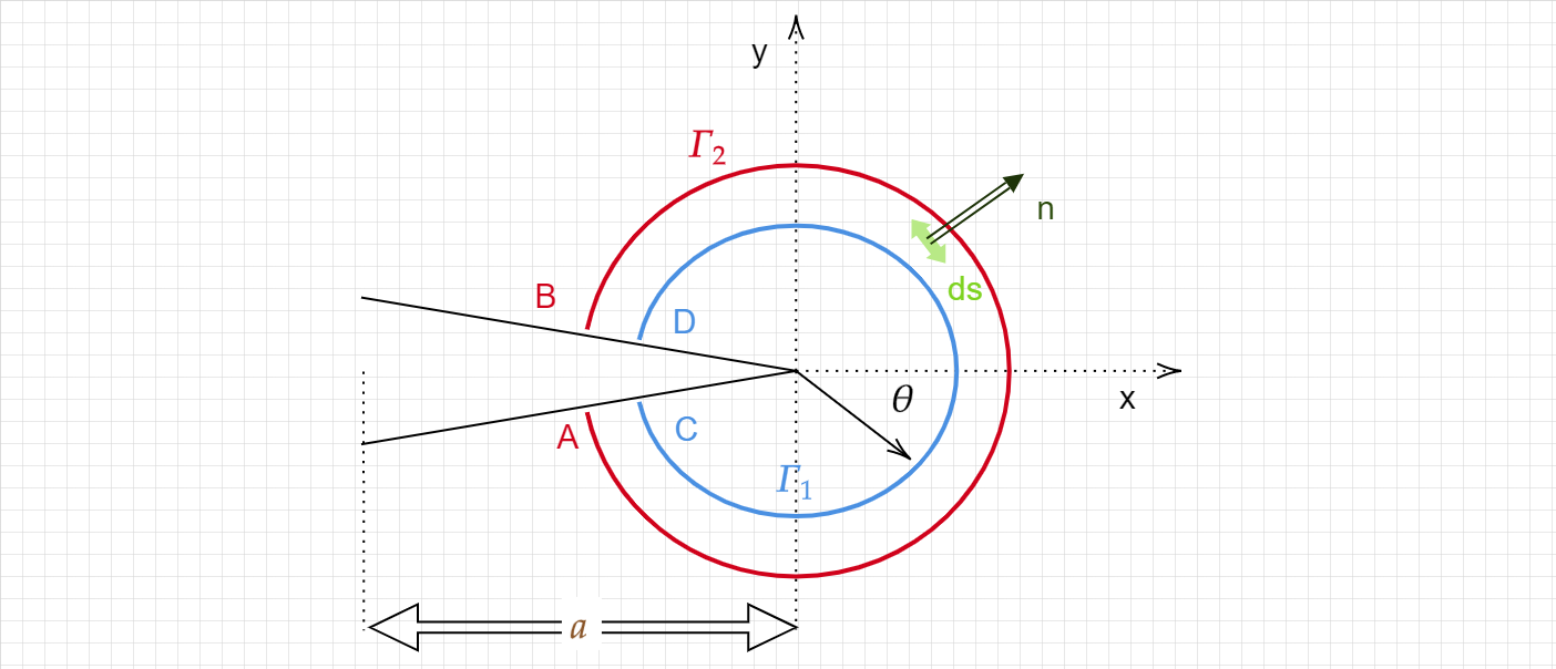
The \(J\) integral is path independent and thus if we integrate along the closed contour defined by \(A,B,C,D\) (i.e. along the blue contour and coming back along the red contour ) we should find the integral to be zero.

The \(J\) integral is being used as a measure of toughness in many structural alloys and industrial applications. For an elastic material (or under SSY assumption) \(J=G\) . For large scale yielding, \(J\) is no longer equal to \(G\) and allow us to extract the toughness of materials which are too ductile for ASTM E399.

Let us try to follow the main steps in deriving the \(J\) integral.

We restrict ourselves to small strains as we will use the \(J_2\) deformation theory of plasticity, which is equivalent to a non-linear elastic formulation, but as long as the loading is proportional and no unloading is concerned, the deformation theory is equivalent to the flow theory of plasticity.

In what to follow we also assume that :

No inertia or body forces exist.
No thermal loading
The crack faces are stress free

As we saw before, the potential energy can be written as :

\[ U=\int_A WdA - \int_S \vec T \cdot u ds \]

Taking the derivative of \(U\) with respect to \(a\) we easily obtain

\[ -\frac{d U}{da} = \int_S \left( Wdy - \vec T\cdot \frac{\partial \vec u}{\partial x} \right) = J \]

Following this derivation, we can understand that \(J\) represent the change in energy resulting from crack growth (just like the energy release rate) however it is derived for a non-linear material.

Note

For the case of a linear elastic material :

\[ J = G = \frac{K^2}{E`} \]

It is actually quite straightforward to show that the \(J\) integral, for the 2D scenario defined above is path independent.

We start be considering the \(J\) integral over am arbitrary closed cycle.

Using Gauss’s theorem we can switch from a line integral to a surface integral such that

\[\begin{split} J = \int_A \left [ \frac{\partial W}{\partial x} -{\color{orange}{\frac{\partial}{\partial x_j}\left( \sigma_{ij} \frac{\partial u_i}{x}\right)}} \right] dxdy \\ \ \ \\ \text{ recall that:} \\ \ \ \\ \frac{\partial W}{\partial x}=\sigma_{ij}\frac{\partial \epsilon_{ij}}{\partial x} \ \ \text{assuming that:} \ \ \frac{\partial W}{\partial \epsilon_{ij}} = \sigma_{ij} \end{split}\]

Next, we can use the small strain assumption which leads to

\[ \frac{\partial W}{\partial x}=\sigma_{ij}\frac{\partial }{\partial x_j} \frac{\partial u_i}{\partial x} \]

(recall that for isotropic materials \(\left( \sigma_{ij}=\sigma_{ji} \right )\) )

using the equilibrium condition \(\left( \frac{\partial \sigma_{ij}}{\partial x_j}=0 \right )\) will leave us with

\[ \frac{\partial W}{\partial x} =\color{orange}{ \frac{\partial }{\partial x_j} \left( \sigma_{ij} \frac{\partial u_i}{\partial x} \right)} \]

and now we know that \(J=0\) for a closed contour.

No, let’s calculate \(J\) over the trajectory defined by \(ABDC\). Since the segments \(\color{red}{A}\color{blue}{C}\) and \(\color{blue}{D}\color{red}{B}\) are traction free we have

\[ J_{\color{red}{A}\color{blue}{C}}=J_{\color{blue}{D}\color{red}{B}}=0 \]

So looking back at the integral going through \(\color{red}{A}\color{blue}{C}{\color{blue}{D}}\color{red}{B}\) we have :

\[ J_{\color{red}{A}\color{blue}{C}}+J_{{\color{blue}{D}}\color{red}{B}} + J_{\color{red}{AB}}-J_{{\color{blue}{DC}}} =0=J_{\color{red}{AB}}-J_{{\color{blue}{DC}}} \Rightarrow J_{\color{red}{AB}}=J_{{\color{blue}{DC}}} \]

Let’s try to estimate \(J\) for a mode III loading.

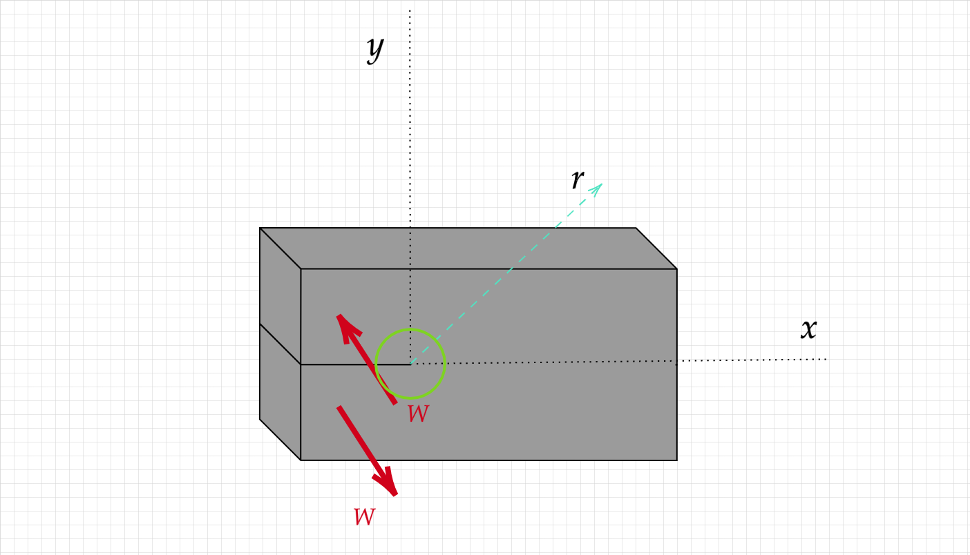
Using what we learned so far, the stress and displacements field can be written as

\[\begin{split} \sigma_{rz}= \frac{K_{III}}{\sqrt {2 \pi r}} \sin \left( \frac{\theta}{2}\right) \\ \\ \ \ \\ \sigma_{z\theta}= \frac{K_{III}}{\sqrt {2 \pi r}} \cos \left( \frac{\theta}{2}\right) \\ \ \ \\ W(r,\theta) = 2\frac{K_{III}}{\mu} \sqrt{\frac{r}{2\pi}} \sin \left( \frac{\theta}{2}\right ) \end{split}\]

To make our life simpler, lets rewrite \(J\) as the sum of two integrals :

\[ J =J_a + J_b = \int_{\Gamma}Wdy - \int_{\Gamma}\vec T \frac{\partial \vec u}{\partial x}ds \]

Starting with \(J_a\) we can calculate the strain energy to be :

\[ W = \sigma_{rz}\epsilon_{rz} + \sigma_{\theta z}\epsilon_{\theta z} = \frac{1}{2 \mu} \left(\sigma_{rz}^2 + \sigma_{\theta z}^2 \right) \]

and using \(dy = ds\cos \theta = r\cos \theta d\theta\) \(J_a\) becomes:

\[ J_a = \int_{-\pi}^{\pi} \frac{1}{2 \mu} \left(\sigma_{rz}^2 + \sigma_{\theta z}^2 \right) r\cos \theta d\theta = 0 \]

Now, we need to examine \(J_b\). For that purpose, we need to calculate the dot product of the tractions on the contour and the outward pointing normal along the route.

Since the only stresses are \(\sigma_{z \theta};\sigma_{rz}\) and the outwards pointing normal is infact aligned with \(\vec{r}\) we are left with :

\[ T_z = \sigma_{rz} = \frac{K_{III}}{\sqrt {2 \pi r}} \sin \left( \frac{\theta}{2}\right) \]

and the derivative of the displacement \(W\) with \(x\) is given by:

\[ \frac{\partial W}{\partial x} = \frac{\partial W}{\partial r} \cos \theta - \frac{1}{r} \frac{\partial W}{\partial \theta} \sin \theta = -\frac{K_{III}}{2 \mu} \sqrt{\frac{2}{\pi r}}\sin \left( \frac{\theta}{2}\right ) \]

After integration (from \(-\pi\) to \(\pi\)) we obtain:

\[ J=\frac{K_{III}^2}{2\mu} \]

Which is exactly the same as \(G\) under mode III.

Note

Measuring \(J\), and not \(K\) relaxes the restrictions regarding the test validity. For a bend specimen, the ASTM requirment is for the ligament (\(b\)) to be \(b>25\frac{2J}{\sigma_y+\sigma_u}\) and \(b>200\frac{2J}{\sigma_y+\sigma_u}\)

FM036004-Notes

The J Integral¶