2. SN Curves¶

2.1. Cyclic fatigue with constant amplitude (\(\sigma\) based)¶

A Wöhler curve, or S-N curve, in its basic form, represent the number of cycles \(N_f\) which will lead to failure, given that the material was loaded with a given stress amplitude

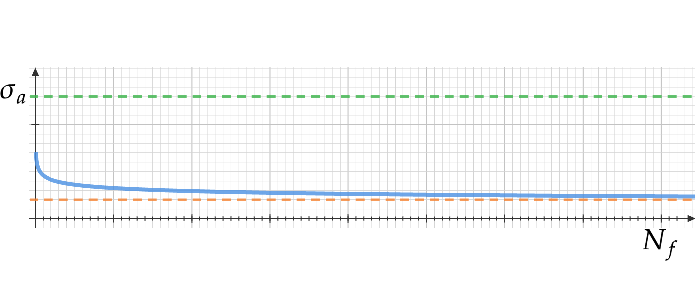
the red line represent the fatigue limit of the material \(\to\) the stress below which an infinite amount of cycles is allowed.

Infinity in the context of fatigue is often set as \(N=10^7\).

For many materials, a linear relation was observed between \(log(\sigma_a)\) and \(log(2N_f)\) , This relation, was proposed by Basquin in 1910 to follow:

\[ \frac{\color{blue}{\Delta \sigma}}{2} = \sigma_a = \sigma'(2N_f)^b \]

where \(\sigma'\) is usually taken as the failure stress of the material and \(b\) is in the empirical range of \([-0.05, -0.12]\)

A missingf piece of this approach as dicussed so far is the assumption that \(\sigma_m = 0\)

Several models have been proposed to handle that, but we will only mention two of them:

Soderberg (1939,more conservative):

\(\sigma_a = \sigma_a^{(\sigma_m=0)} \left ( 1-\frac{\sigma_m}{\sigma_y} \right )\)

Goodman(1899):

\(\sigma_a = \sigma_a^{(\sigma_m=0)} \left ( 1-\frac{\sigma_m}{\sigma_{UTS}} \right )\)

2.2. Cyclic fatigue with varying amplitude (\(\sigma\) based)¶

For many real life scenarios (e.g. estimating life of aircraft components, dental implants etc.) it makes more sense to subject the test specimen to a spectrum load which represent in a more realistic way the loads it will experience throughout its life cycle.

To account for the varying amplitude (amongst others) we can use \(Miner's rule\) which can be written as:

\[ D=\sum_i d_i=\sum_i \frac{n_i}{N_{fi}} \]

As long as \(D<1\) the component is persumabley safe.

Note

Miner’s rule does not take under consideration the order in which the different loading cycles were applied.

Why is that a major drawback?

Strain hardening/softening
\(\mu\)-cracks nucleation

2.3. Low cycle fatigue (\(\epsilon\) based)¶

For scenarios where significant plasticity might occur, we will prefer to take a strain based approach (high temperature, locally high stresses etc. )

by plotting \(\frac{1}{2}\Delta \epsilon^p\) vs \(2N_f\) we will again observe(usually) a linear relation described by (Coffin Manson 1955):

\[ \frac{\Delta \epsilon^p}{2}=\epsilon_f'(2N_f)^c \]

where \(c\) lies in the range of \([-0.5,-0.7]\) (empirically).

If we combine the stress approach (Basquin) with the strain one we can use simple linear elasticity to obtain

\[ \frac{1}{2}\Delta \epsilon^e = \frac{1}{2}\frac{\Delta \sigma }{E} = \frac{\sigma'}{E}(2N_f)^b \]

and after substitution:

\[ \frac{\Delta \epsilon}{2}=\epsilon_f'(2N_f)^c+\frac{\sigma'}{E}(2N_f)^b \]

Moreover, we can find the transition between elastic and plastic dominant scenarios by taling the two terms to be equall yielding:

\[ 2N_t = \left (\frac{E\epsilon_f'}{\sigma'} \right )^{1/(b-c)} \]

2.4. Lies damn lies and statistics¶

The scatter observed in fatigue tests tend to be rather large, with \(N_f(\sigma_f)\) exhibiting a log-normal distribution and \(\sigma_f(N_f)\) a normal distribution.

One of the issues arising when dealing with fatigue tests on smooth specimens is theat the crack initiation stage may take up a large portion of \(N_f\).

It is sensitive to effects such as:

grain orientation near the surface
inclusions distribution as a function of \(r\)
defects population in general
machinning defects

2.4.1. Cyclic hardening/softening¶

many structural alloys will exhibit cyclic strain hardening (both isotropic and kinematic). For some alloys this will only be present n the first few cycles before saturating, and in some cases, a maximum will be attained which will later decrease before saturating.

Similarly, some materials (e.g. low carbon steels) exhibit softening acompanying heterogenous strainning followed by hardening with homogenous deformation.

FM036004-Notes