Crack Tip Plasticity¶

In the previous lecture we derived the stress in the vicinity of a crack in an elastic body. As you may recall, the asymptotic solution contained a $\frac{1}{\sqrt{r}}$ singularity, which in turn should result in an infinite stress.

AS we mentioned briefly, an infinite stress is ok as long as we are within the framework of LEFM. Otherwise, we can expect material non-linearities to play a role once sufficient levels of stress/strain energy are involved.

One such non-linear behavior you are all acquainted with is plasticity.

Before starting our discussion regarding Crack Tip plasticity Lets take a moment to remember what plasticity is. This will accompany us in future lessons so please stop me if anything is unclear !

Plasticity in a nutshell¶

We will focus our discussion on small strain, rate and temperature independent plasticity.

This section is by no means aimed at teaching plasticity but rather its purpose is to get us all on terms regarding some very basic concepts which we will be using in the sections to follow.

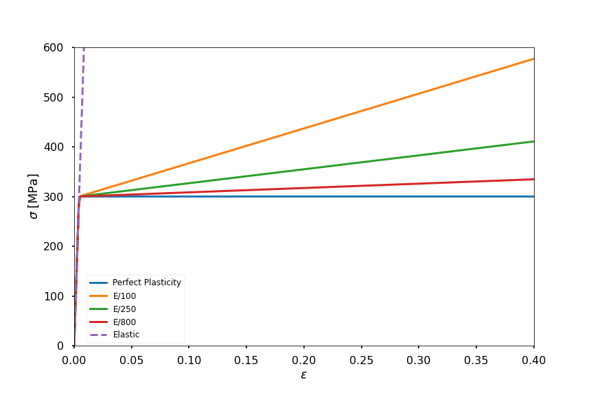
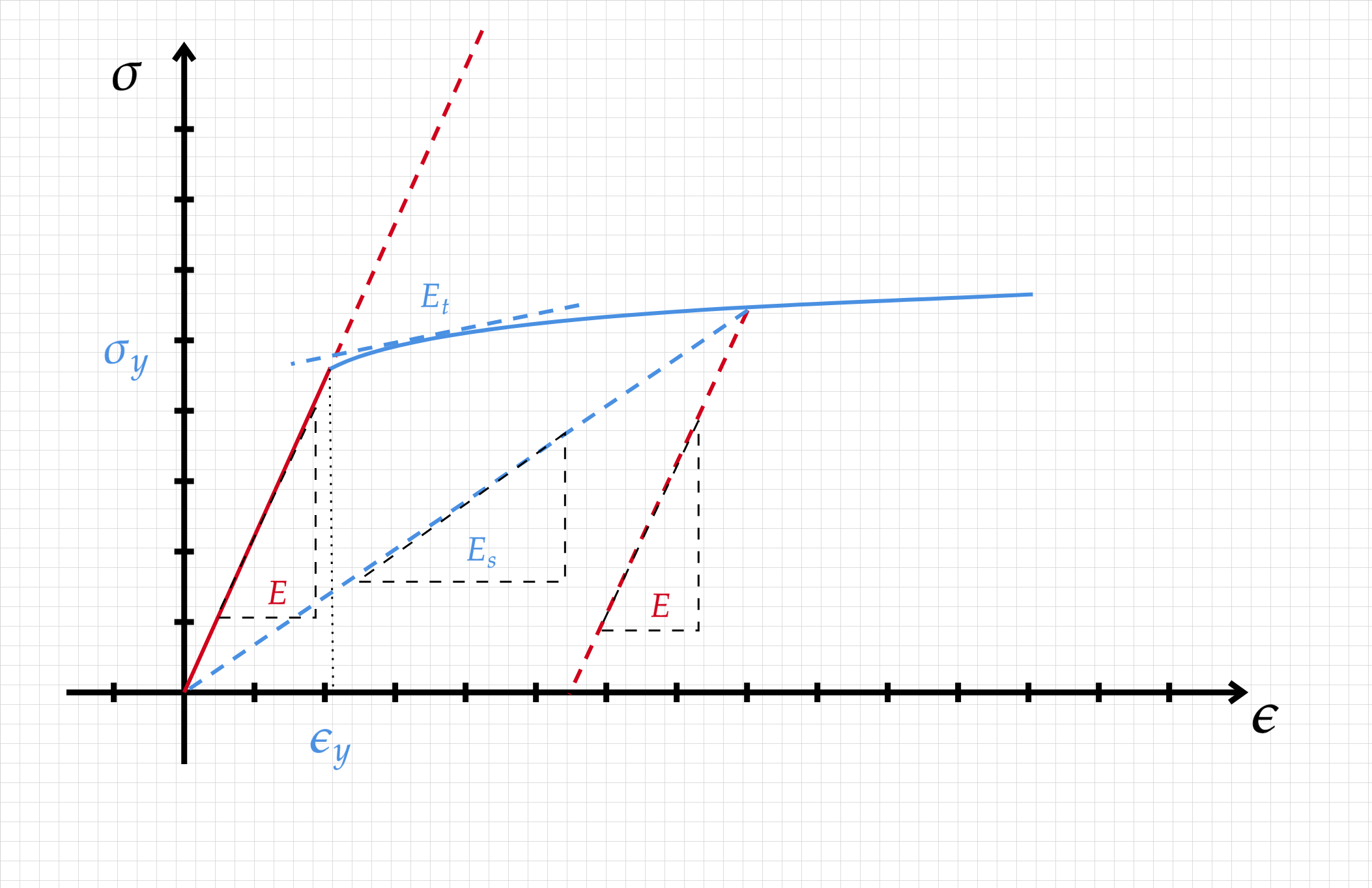
We are all used to looking at the plots below when considering the mechanical behavior of metals.

Among the many hardenning rules you can find in the literature, we will focus on just three:

Perfect plasticity - once the material has yielded it will continue to flow at the same stress as the yielding stress :

\[\begin{split} \sigma = \begin{cases} E \epsilon \ \ &; \ \ \epsilon<\epsilon_y \\ \sigma_y \ \ &; \ \ \epsilon \geq \epsilon_y \end{cases} \end{split}\]
Linear hardening -

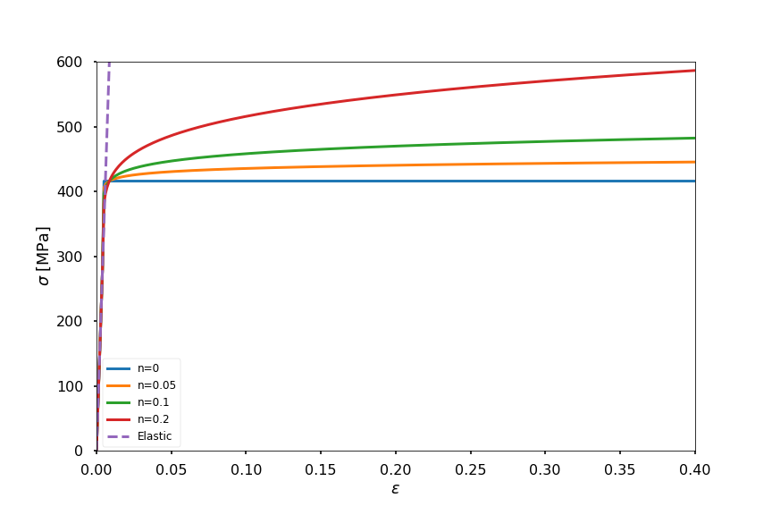
\[\begin{split} \sigma = \begin{cases} E \epsilon \ \ &; \ \ \epsilon<\epsilon_y \\ \sigma_y+ K(\epsilon-\epsilon_y) \ \ &; \ \ \epsilon \geq \epsilon_y \end{cases} \end{split}\]
Power law hardening

\[\begin{split} \sigma = \begin{cases} E \epsilon \ \ &; \ \ \epsilon<\epsilon_y \\ \sigma_y+ K(\epsilon-\epsilon_y)^n \ \ &; \ \ \epsilon \geq \epsilon_y \end{cases} \end{split}\]

And we all remember that the yield stress $\sigma_y$ is determined by the stress at $0.02\%$ strain.

This is of course an engineering convention which allow us to communicate.

However it s good to keep in mind that plasticity (e.g. dislocation movement) starts at much lower stresses, it just happens at a scale that we are not accustomed to measure or think about in the context of continuum mechanics.

We will talk about it more when discussing fatigue.

So what is plasticity

Plasticity occurs through the nucleation, movement and interaction of defects. We will elaborate on those mechanisms in future sessions.

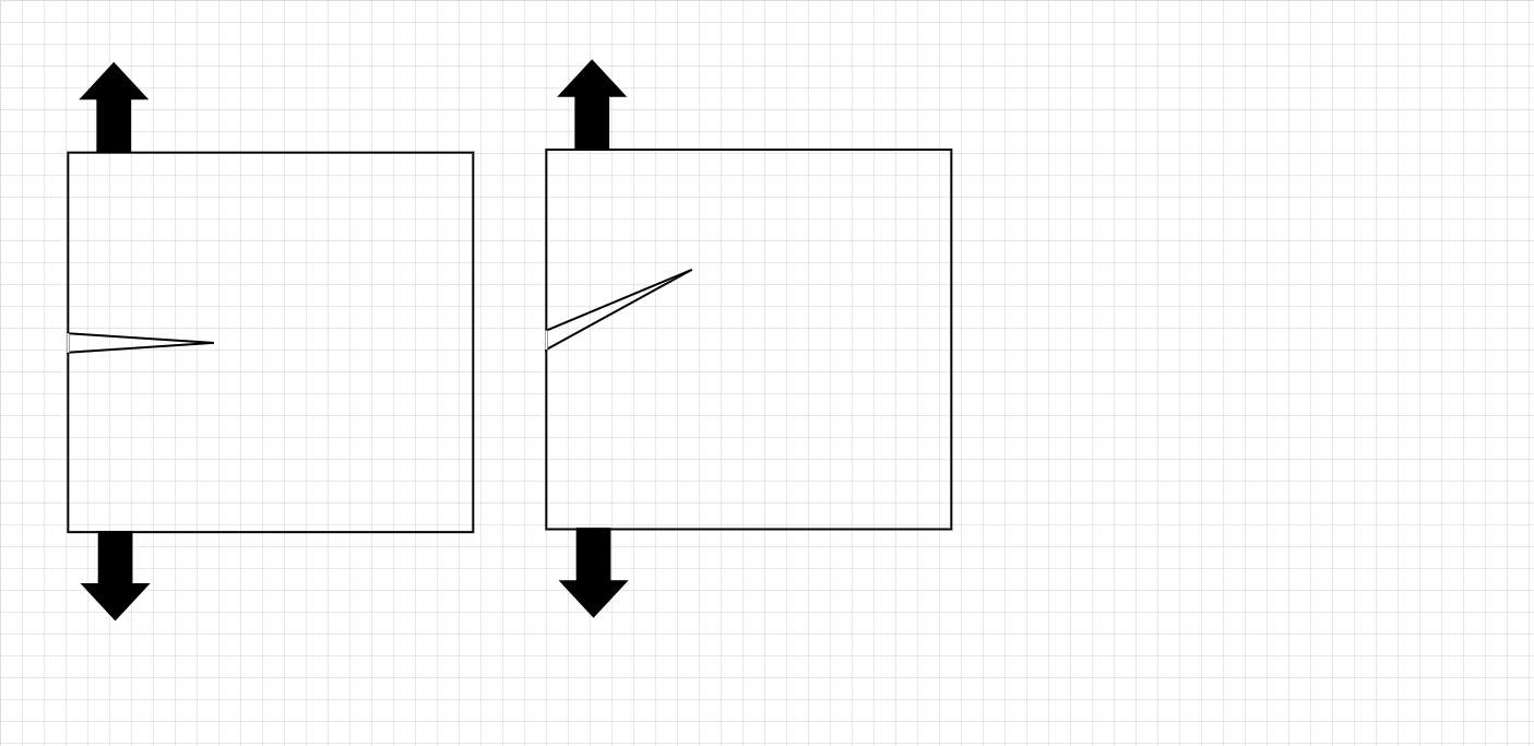
When conducting a uniaxial test, plasticity is manifested as a transition from the linear behavior of linear elasticity.
Once the stress exceeds a critical value, a permanent change in shape will take place.
The total measured strain is the sum of the elastic and plastic contributions such that:

\[\begin{split} d\epsilon_{ij} = d\epsilon_{ij}^e + d\epsilon_{ij}^p \\ \end{split}\]
Upon unloading, the $\sigma - \epsilon$ curve will follow the same slope as the elastic loading curve (assuming no damage). following this statement we can write:

\[ d\sigma_{ij} = \mathbb{C}_{ijkl}d\epsilon^e_{ij} \]
Plasticity by itself is independent on the magnitude of applied hydrostatic stresses (those will result in volume change which belongs to the realm of elasticity), leading to :

\[ \dot{\epsilon_{kk}^p} = 0 \]
Under multi-axial conditions, whether plasticity will take place or not is determined using a yield surface/criteria.
The evolution of the yield surface is determined by a **flow rule ** (strain hardening)
Finally, unlike linear elasticity where the initial and final configuration determined the stress state, regardless of the path between them, plasticity is path dependent.

In general, it is convenient to define the yield criteria using

\[ f(J_2,J_3,\bar{\epsilon}^p)=k-Y(\bar{\epsilon}^p)=0 \]

With $J_i$ being the invariants of the deviatoric stress tensor $S_{ij}$ defined as:

\[ S_{ij} = \sigma_{ij} - \frac{1}{3}\sigma_{kk} \]

and its invariants are:

\[\begin{split} J_1 = 0 \ \ \text{plasticity is volume conserving}\\ J_2 = \frac{1}{2}S_{ij}{S_ij} \rightarrow \sigma_e = \sqrt{3J_2}\\ J_3 = det(\mathbb{S}) \end{split}\]

You have already encountered the concept of plastic yielding before and phrased the yield criteria as either the Tresca criteria or the Levy Von Mises criteria.

\[\begin{split} \textbf{Tresca}\\ f(\sigma_{ij},\bar{\epsilon}^p) = 0 = \max \left[|\sigma_1 - \sigma_2|;|\sigma_1 - \sigma_3|;|\sigma_2 - \sigma_3| \right] -Y(\bar{\epsilon}^p) \end{split}\]

\[\begin{split} \textbf{Levy Von Mises}\\ f(\sigma_{ij},\bar{\epsilon}^p)= 0 =\sqrt{\frac{3}{2}S_{ij}S_{ij}}-Y(\bar{\epsilon}^p) \end{split}\]

The equivalent plastic strain $\bar{\epsilon}^p$ is given by :

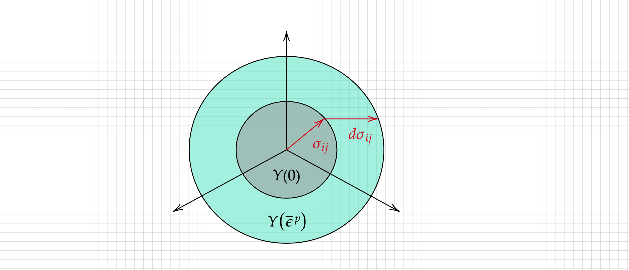
\[ \bar{\epsilon}^p = \int \sqrt{\frac{2}{3}d\epsilon_{ij}^p d\epsilon_{ij}^p} \]

The flow rules attached to the yield criteria above are termed isotropic as the yield surface is growing proportionally in all direction

Question

How the evolution of the yield surface relates to the cyclic behavior we will observe when cycling between tensile and compressive loads?

the increment of plastic strain $d\epsilon_{ij}^p$ is given by :

\[ d\epsilon_{ij}^p = \frac{3}{2}d\bar{\epsilon}^p \frac{S_ij}{Y(\bar{\epsilon}^p)} \]

and $d\bar{\epsilon}^p$ is easily obtained from the yield surface following:

\[\begin{split} f(\sigma_{ij}+d\sigma_{ij},\bar{\epsilon}^p+d\bar{\epsilon}^p) = f + \frac{\partial f}{\partial \sigma_{ij}}d\sigma_{ij} + \frac{\partial f}{\partial \bar{\epsilon}^p}d\bar{\epsilon}^p =0 \\ \text{since } f \text{ is 0 by definition we obtain that}\\ \frac{\partial f}{\partial \sigma_{ij}}d\sigma_{ij} =- \frac{\partial f}{\partial \bar{\epsilon}^p}d\bar{\epsilon}^p \end{split}\]

The effect of isotropic hardening on the yield surface is outlined below:

Another form of strain hardening is kinematic hardening in which the yield surface does not change it size but rather translates its origin in the stress space :

\[ f(\sigma_{ij},\alpha_{ij}) = 0 = \sqrt{\frac{3}{2}(S_{ij}-\alpha_{ij})(S_{ij}-\alpha_{ij})}-Y \]

and

\[ d{\epsilon}_{ij}^p = \frac{3}{2}\frac{S_{ij}-\alpha_{ij}}{Y}d\bar{\epsilon}^p \]

Question

And now? how the evolution of the yield surface relates to the cyclic behavior we will observe when cycling between tensile and compressive loads?

Flow vs. Deformation theories - illustrated¶

Yielding at the crack tip¶

The plastic zone size¶

We will examine two approaches for evaluating the size of the plastic zone - $\color{blue}{r_p}$

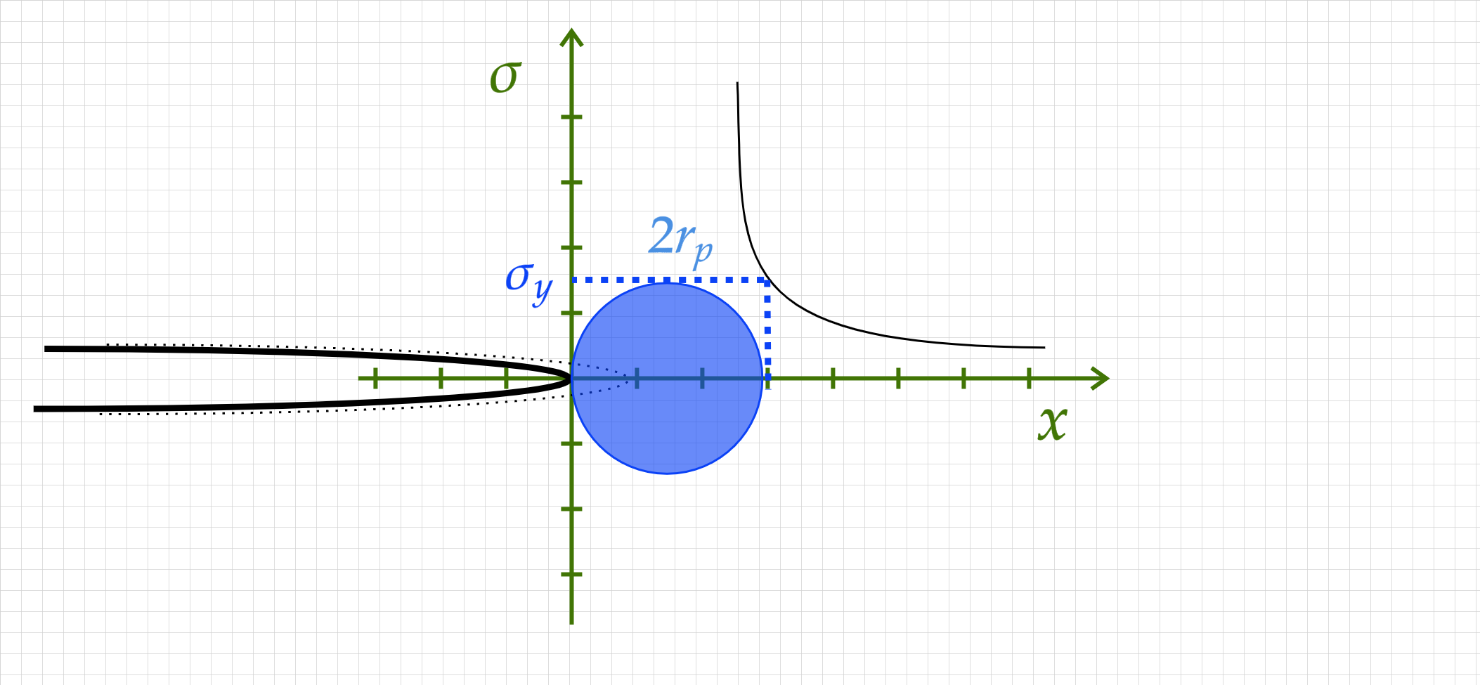
The Irwin plastic zone size¶

Irwin’s approach for estimating the plastic zone size is based on equating the stress component $\sigma_{yy}$ with the yield stress $\color{blue}{\sigma_y}$ on the crack plane. We assume a non-hardening material and plane stress conditions (can you guess why?).

from the above we obtain :

\[ {\color{blue}{r_p}}=\frac{1}{2\pi}\left (\frac{K_I}{\color{blue}{\sigma_y}} \right)^2 \]

To get a better approximation, accounting for the yielding and re-arrangement of stresses we will look at the balance of forces in the region which undergoes yielding :

\[ {\color{blue}{\sigma_y r_p}}= \int_0^{\color{blue}{r_p}}\sigma_{yy}dr=\int_0^{\color{blue}{r_p}}\frac{K_I}{\sqrt{2\pi r}}dr \Longrightarrow {\color{blue}{r_p}}=\frac{1}{\pi}\left( \frac{K_I}{{\color{blue}{\sigma_y}}}\right)^2 \]

To account for the lower stresses in the plastic zone (remember plasticity is a softening mechanism), Irwin proposed to use a fictitious crack length such that

\[ a_{eff} = a+\color{blue}{r_p} \]

where for plane stress $\color{blue}{r_p}$ is given by the above $1^{st}$ order approximation.

For plane strain we need to consider the effect of stress triaxiality, leading to :

\[ {\color{blue}{r_p}}=\frac{1}{6\pi}\left (\frac{K_I}{\color{blue}{\sigma_y}} \right)^2 \]

armed with these expressions we can now estimate the effect of yielding at the crack tip on the stress intensity factor for any geometry ($Y$ is geometry dependent) using:

\[ K_{eff} = Y(a_{eff})\sigma\sqrt{\pi a_{eff}} \]

Obtaining the actual solution is done iteratively :

Find $K$ assuming only elasticity
Use the obtained $K$ to estimate $\color{blue}{r_p}$ and $a_{eff}$
Calculate $K_{eff}$
Re-calculate $K_{eff}$ using the newly found $a_{eff}$
Continue until convergence

For some limited number of cases a closed form solution exists.

The Dugdale Barenblatt strip model¶

Here we will make use of the same concept of closure stress as we did in the previous lecture.

We will start by looking at an infinite plate with a through crack made of an elastic-perfectly plastic material.

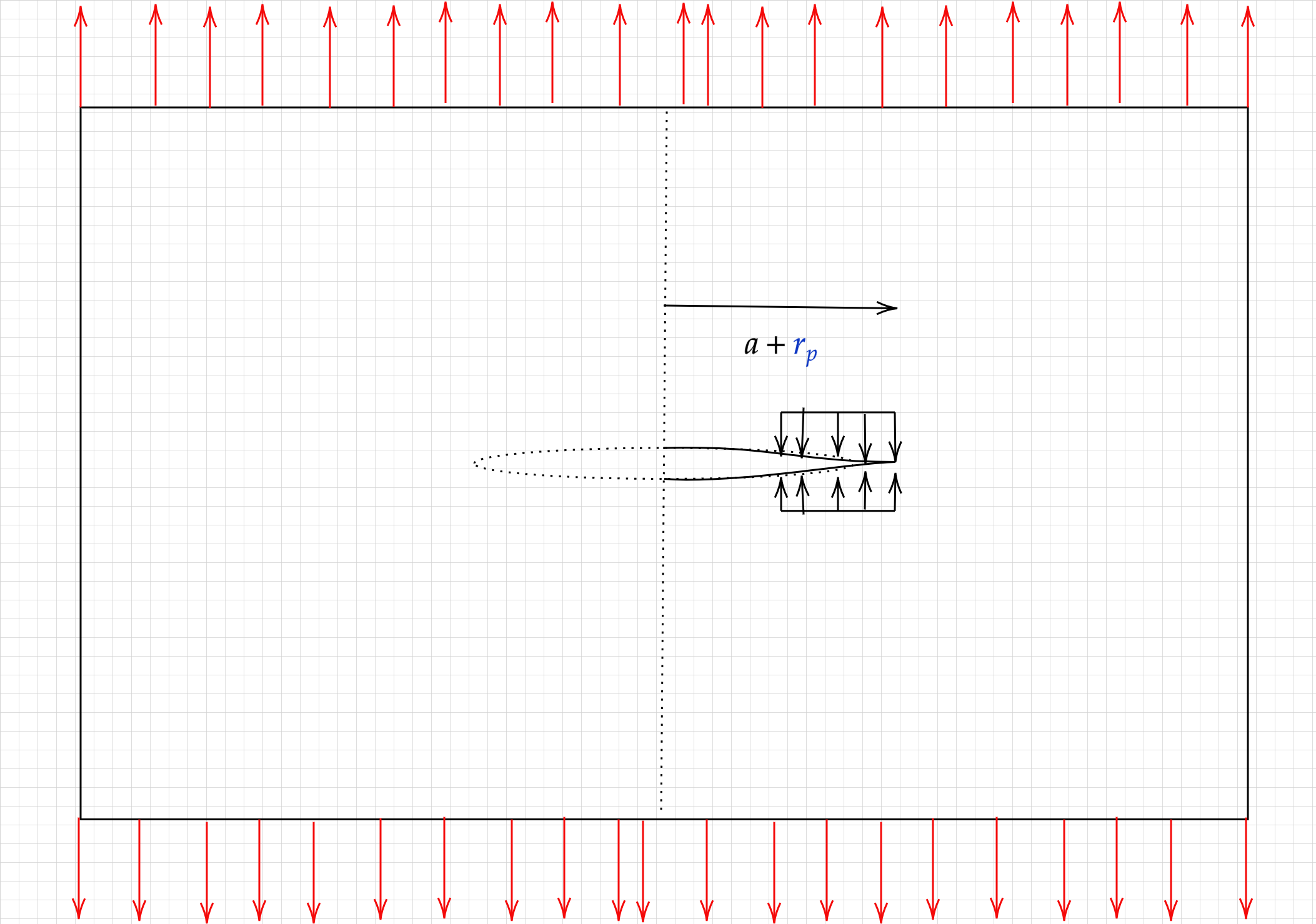
In the figure above, the stresses acting to close the crack tip are given by $\color{blue}{\sigma_y}$ and are finite. there can be no $1/\sqrt{r}$ singularity in the stress field and thus the first term in the series expansion must be zero.

In other words, we are now tasked with finding $\color{blue}{r_p}$ such that the stress intensity arising from the reote tensile field and the one arising from the application of the closure stress will cancel out.

\[\begin{split} K_{+a} = \frac{P}{\sqrt \pi a}\sqrt{\frac{a+x}{a-x}} \\ K_{-a} = \frac{P}{\sqrt \pi a}\sqrt{\frac{a-x}{a+x}} \end{split}\]

and

\[ P=-{\color{blue}{\sigma_y}}dx \]

replacing $a$ in the expressions for $K_{\pm a}$ with $a+\color{blue}{r_p}$ , summing the two terms and integrating over the part of the crack being subjected to closure stress ($a \rightarrow a+\color{blue}{r_p}$) leads to :

\[ {\color{green}{K_{closure}}} = -2{\color{blue}{\sigma_y}}\sqrt{\frac{a+{\color{blue}{r_p}}}{\pi}}\cos^{-1}\frac{a}{a+{\color{blue}{r_p}}} \]

Next, by demanding the the $\color{red}{K}$ resulting from the remote tensile load will be equal to $\color{green}{K_{closure}}$ we obtain

\[ {\color{green}{K_{closure}}} = -2{\color{blue}{\sigma_y}}\sqrt{\frac{a+{\color{blue}{r_p}}}{\pi}}\cos^{-1}\frac{a}{a+{\color{blue}{r_p}}}= {\color{red}{K_{remote}}}={\color{red}\sigma_{\infty}}\sqrt{\pi (a+{\color{blue}{r_p}})} \]

leading to

\[ \frac{a}{a+{\color{blue}r_p}}=\cos \left( \frac{\pi {\color{red}\sigma_{\infty}}}{2{\color{blue}\sigma_y}}\right) \]

Question…

What happens when $${\color{red}{\sigma_{\infty}}}={\color{blue}{\sigma_y}}$$

Almost done..

All that’s left is to expand the last expression using a Taylor series expansion, and look at the limit where ${\color{red}\sigma_{\infty}}<< {\color{blue}\sigma_y}$ :

\[ {\color{blue}r_p} = \frac{\pi}{8}\left (\frac{\pi{\color{red}{\sigma_{\infty}}}^2a}{{\color{blue}{\sigma_y}}^2}\right) \]

Note

Note that the Dugdale Barenblatt expression and the Irwin expression only differ by their prefactor $1/\pi$ compared to $\pi/8$

Finally by plugging $a+{\color{blue}r_p}$ into the “usual” expression for $K_I$ we obtain

\[ {\color{blue}{K_{eff}} }={\color{red}\sigma_{\infty}}\sqrt{\pi a \sec\left(\frac{\pi {\color{red}\sigma_{\infty}}}{2{\color{blue}\sigma_y}} \right) } \]

As in Irwin’s model, the strip model does not account for strain hardening and tends to overestimate ${\color{blue}r_p}$ resulting in an overestimation of $K$.

The plastic zone shape¶

So far we discussed what happens upon yielding (locally) for $\theta=0$. But what happens away from the symmetry plane?

The principal stresses for a mode I crack (asymptotic solution) are given by:

\[\begin{split} \sigma_1 = \frac{K_I}{\sqrt{2\pi r}}\cos\left (\frac{\theta}{2}\right )\left[1+\sin\left (\frac{\theta}{2}\right )\right]\\ \sigma_2 = \frac{K_I}{\sqrt{2\pi r}}\cos\left (\frac{\theta}{2}\right )\left[1-\sin\left (\frac{\theta}{2}\right )\right]\\ \sigma_3 =\begin{cases} 0, \ \ \text{plane stress}\\ \frac{2 \nu K_I}{\sqrt{2\pi r}}\cos\left (\frac{\theta}{2}\right ),\ \ \text{plane strain} \end{cases} \end{split}\]

We can construct $\sigma_e$ using the three principal stresses and isolate $\color{blue}r_p$ by setting $\sigma_e={\color{blue}\sigma_y}$ to obtain the relation between the plastic zone size and the angle $\theta$:

\[\begin{split} {\color{blue}r_p}(\theta)=\begin{cases} \frac{1}{4\pi}\left ( \frac{K_I}{{\color{blue}\sigma_y}}\right)^2\left [ \left(1-2\nu\right)^2(1+\cos\theta)+\frac{3}{2}\sin^2\theta\right], \ \ &\text{plane strain}\\ \frac{1}{4\pi}\left ( \frac{K_I}{{\color{blue}\sigma_y}}\right)^2\left [ 1+\cos\theta+\frac{3}{2}\sin^2\theta\right], \ \ &\text{plane stress} \end{cases} \end{split}\]

FM036004-Notes