16. Analysis of Experimental Measurments¶

Once we gathered all the experimental data we were looking for it is time to put this information to use.

However, prior to doing so, we need to understand the limitations of our data. In previousl lectures, we discussed how to gather the information properly, using calibration, proper sampling, and noise reduction techniques.

Now, we will try to put the information we obtained from the experiments in a different context, trying to answer questions such as:

Does the gathered data (based on a finite number of measurments) pose a good approximation for the population as a whole?
How can we represent the entire data set using a minimal set of values?
How can we test the hypothesis we had prior to performing the experiment?
Can we be sure that we will meet the required tolerances, given the scatter in our data?
Does it make sense at all?

As you can guess, our focus will be on random errors and we will assume (for now) that we have eliminated all other sources of error we can think of. This assumption will of course ve tested during the analysis we will conduct.

import numpy as np 
import pandas as pd
import matplotlib.pyplot as plt
from matplotlib.font_manager import FontProperties
from matplotlib import rcParams
plt.style.use('fivethirtyeight')
plt.ion()
%matplotlib inline
rcParams["figure.figsize"] = [12, 8]

---------------------------------------------------------------------------
ModuleNotFoundError                       Traceback (most recent call last)
Input In [1], in <cell line: 2>()
      1 import numpy as np 
----> 2 import pandas as pd
      3 import matplotlib.pyplot as plt
      4 from matplotlib.font_manager import FontProperties

ModuleNotFoundError: No module named 'pandas'

16.1. Probability¶

We have previously used expressions such as:

\[ X \pm \mu \]

where we reffered to $\mu$ as the uncertainty. Lets focus on that for a few minutes.

What does an uncertainty of $\mu$ actually means?

For simplicity let us consider a general case, where we are measuring a physical quantity $X$. When reporting the value of $X$ we actually report a probable value. In other words we will report something like:

\[ X=\bar{X}\pm \mu \ \ (T_{\mu}) \]

here, $X$ is what we are looking for, $\bar{X}$ is the most probable value for $X$ and $\pm \mu$ is the uncertainty interval with a probability $T_{\mu}$.

Since we can (almost) never sample the entire population, we use the observations (sample) we have and try to draw conclusions from it.

So when we reported $\bar{X}$ we were refering to the sample mean.

\[ \bar{X} = \frac{1}{n}\sum_{i=1}^n X_i \]

That was simple.

But, what does $\pm \mu$ means and how do we associate it with $T_{\mu}$?

$\mu$ is the sample standard deviation, which we estimate by measuring the distance between our observations and the sample mean.

\[ \mu = \left[ \frac{1}{n-1}\sum_{i=1}^n \left(X_i-\bar{X}\right )^2 \right]^{1/2} \]

Before discussing how we obtain $T_{\mu}$ and why did we define $\mu$ the way we did, lets revise reall quick what you know from your course in probability and statistics.

Probability function

Given a smapling space $\Omega$ of discrete values, the probability function $P$ maps each discrete value $x_i$ to a number between $0$ and $1$ such that $0 \leq P(x_i)\leq 1$ and $\sum_i P(x_i) =1$

Without getting into details we will remind ourselves that :

$P(A \cup B) = P(A) +P(B) - P(A \cap B)$
$P(A|B) $ is the probability of $A$ given that $B$. $P(A|B)=\frac{P(A\cap B)}{P(B)}$
If $A$ is independent of $B$ than $P(A|B)=P(A)$ and $P(A \cap B) = P(A)\cdot P(B)$

We can ow recall Bayes’ rule:

Given two events $A$ and $B$ we can write:

\[ P(B|A) = \frac{P(A|B)\cdot P(B)}{P(A)} \]

The Bayes rule allow us to ask ourselves what is the probability of $B$ happening given that $A$ happens, from knowledge we have regarding the probability of $A$ occuring if $B$ happend. in other words it allows us to reverse the direction of the conditional probability.

Example

We ordered a set of cooling elements from three suppliers. (why?) After inserting the units to production we found that some of the units lead to premature falure of our product due to extensive heating:

Supplier	Fraction of stock	$P$ of failed units
A	$P(A)=0.40$	$P(F
B	$P(B)=0.25$	$P(F
C	$P(C)=0.35$	$P(F

We now want to ask our selves what is the probability for a failed product to contain a unit manufactured in $A,B,C$?

The answer is obtained using Bayes rule

First we can find $P(F)=P(F|A)P(A) + P(F|B)P(B) + P(F|C)P(C) = 0.033$ and now

\[\begin{split} P(A|F) = \frac{P(F|A)\cdot P(A)}{P(F)}=\frac{0.025*0.4}{0.033} = 0.303\\ P(A|F) = \frac{P(F|A)\cdot P(A)}{P(F)}=\frac{0.05*0.25}{0.033} = 0.379\\ P(A|F) = \frac{P(F|A)\cdot P(A)}{P(F)}=\frac{0.03*0.35}{0.033} = 0.318 \end{split}\]

Remeber this example as we will revisit it soon when we try to decide which supplier is better for us

To continue with our discussion on probability we will make a distinction between discrete and continous variables and distributions.

16.1.1. Discrete variables¶

Given a discrete variable $X$ we can define $f(x)=P(X=x)$ with $f(x)$ being the probability mass function PMF.

Lets take the first HW grade as our discrete variable.

We plot the number of observations at each grade

grades = pd.read_csv('../rep/grades.csv')

fig, axs = plt.subplots(2,2)

axs[0,0].hist(grades.HW1,bins=100, density=False);
axs[0,1].hist(grades.HW1,bins=10, density=False);
axs[1,0].hist(grades.HW1,bins=100, density=True);
axs[1,1].hist(grades.HW1,bins=10, density=True);

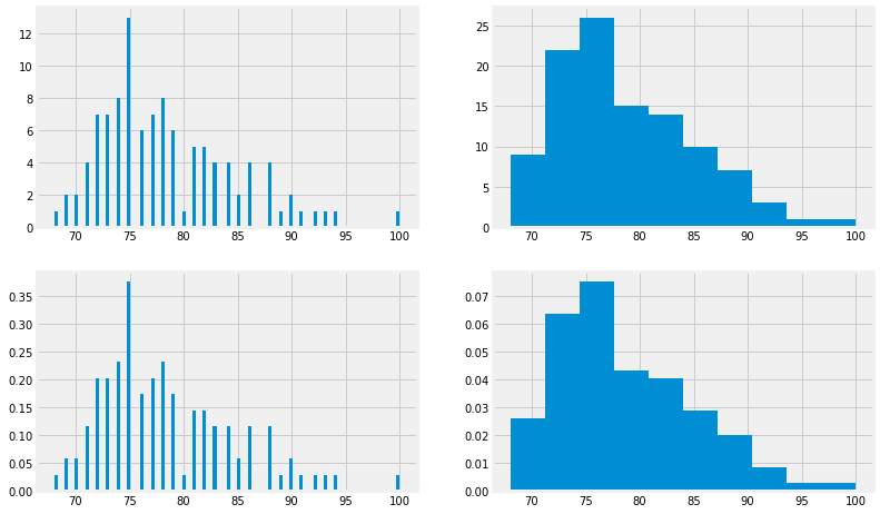
Question

What is the difference between the 4 plots above?
From which plot its easier for you to get a “feel” regarding the course grades?

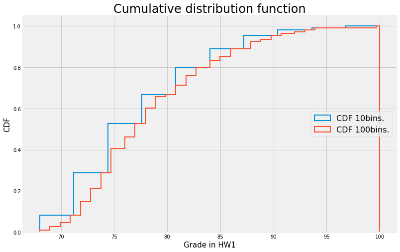
Another way to visualize this data is to look at the cumulative distribution function or CDF

The CDF is defined by $F(t)=P(X \leq t)$

fig, ax = plt.subplots()
ax.hist(grades.HW1, bins=10, density=True, histtype='step', cumulative=1,
        label='CDF 10bins.', linewidth=2)
ax.hist(grades.HW1, bins=100, density=True, histtype='step', cumulative=1,
        label='CDF 100bins.',  linewidth=2)

ax.grid(True)
ax.legend(loc='right',fontsize=16)
ax.set_title('Cumulative distribution function',fontsize=24)
ax.set_xlabel('Grade in HW1',fontsize=15)
ax.set_ylabel('CDF',fontsize=15)

plt.show()

16.1.1.1. Not all distributions are born the same¶

Bernoulli distribution

A Bernoulli distribution is such where the random variable can attain a value of $0$ or $1$ (e.g. pass or fail) . As such $P(X=1)=p$ and $P(x=0)=1-p$

Binomial distribution $B(n,p)$

A binomial distribution answer the questions :

What is the probability to succedd in $n$ independent experiments where all of them are described by the Bernoulli distribution with $p$

Hypergeometric distribution

Similar to the previous distributions, $x$ can take only two values.

Here we are asking the question: Given that we check $n$ units out of a set of $N$ where $K$ units are not meeting the quality standards of our production line. What is the propability that we will check $x$ disqualified units?

\[\begin{split} f(x)=\frac{\begin{pmatrix} K \\ x \end{pmatrix} \begin{pmatrix} N-K \\ n-x \end{pmatrix} }{\begin{pmatrix} N \\ n \end{pmatrix} } \end{split}\]

in case you forgot : $\begin{pmatrix} N \\ n \end{pmatrix} = \frac{N!}{n!(N-n)!}$

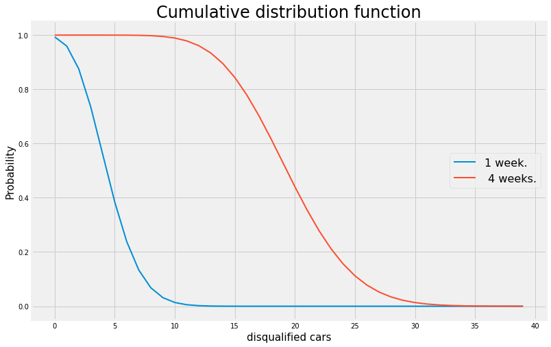
Poisson distribution

Poisson distribution is used to describe the probability of $n$ events occuring over a given duration.

the PMF of a Poisson random variable $X$ is

\[ f(x)=\frac{e^{-\lambda}\lambda^x}{x!} \]

where $\lambda = E(X)=Var(X)$ which is quite convinient :)

Example

Assume that a car manufacturer produces $9615$ cars per week. On avarage, $5$ cars a week are disqualified due to poor workmanship.

what is the probability that next week at least one car will be disqualified?
what is the probability that next week no more than one car will be disqualified
what is the probability that in the next 4 weeks more than 30 cars will be disqualified?

At least one car

We are looking for $$ P(X \geq 1)= 1-P(X=0) = 1-frac{\exp(-5)5^0}{0!} = 0.9933 $$

Maximum one car

\[ P(X\leq 1) = P(0)+P(1) = frac{\exp(-5)5^0}{0!} + frac{\exp(-5)5^1}{1!} = 0.0404 \]

More than $30$ cars in the next $4$ weeks:

SInce we only know the weekly probablity we need to define a new variable that will reffer to what happend over a duration of $4$ weeks. Lets call it $Y$

\[ \lambda_Y = \lambda_X * 4 = 20 \]

and we are looking for $P(Y>30)$ which is the same as $1-P(Y \leq 29)$ An we find that $P(Y>30)= 0.0218$

from scipy.stats import poisson
mu=5
P = poisson(mu)
print(1-P.pmf(0))
print(P.pmf(0)+P.pmf(1))
PY = poisson(mu*4)
print(1-PY.cdf(29))

9932620530009145
040427681994512805
02181821752555746

x=np.arange(0,40,1)

fig, ax = plt.subplots()
ax.plot(x,1-P.cdf(x), label='1 week.', linewidth=2)
ax.plot(x,1-PY.cdf(x), label=' 4 weeks.', linewidth=2)

ax.grid(True)
ax.legend(loc='right',fontsize=16)
ax.set_title('Cumulative distribution function',fontsize=24)
ax.set_xlabel('disqualified cars',fontsize=15)
ax.set_ylabel('Probability',fontsize=15)

plt.show()

16.1.2. The expectation value - characterizing the central tendency¶

Now here it gets tricky. We are used to use $\mu$ for the uncerainty but in probability and statistics it is often used for describing the *mean or expectation value we will use $E(X)=\mu$ interchangably so keep it in mind.

SO, the expectation value (or expected value) of a random discrete variable $X$ sampled $n$ times is given by

\[ E(X)=\sum_{i=1}^N p(x_i)x_i \]

what is $E(X)$ for a Bernouli distribution?
what is $E(X)$ for the binomial distribution?
Can you find an expression for $E(Y)$ with $Y$ being a fnction of $X$?

The sample mean is calculated over our sampled data such that :

\[ \bar{x} = \frac{1}{n}\sum_{i=1}^n x_i \]

16.1.3. The variance - characterizing the spread¶

The population variance, which a measure for how spread are the values of $X$ with respect to $E(X)$ is defined by:

\[ Var(X) = E((X-\mu)^2) = \sigma^2 \]

With $\sigma$ being the standard variation. (note: $Var(X+Y)=Var(X)+Var(Y)$ for independent $X,Y$ )

Similarly, the sample variance $s^2$ is defined over the set of samples we have :

\[ s=\sqrt{\frac{1}{n-1} \sum_{i=1}{n} \left( x_i - \bar{x} \right ) ^2} \]

and $s$ is the standard deviation of the sample.

Note

both $\mu$ and $\sigma^2$ are moments . We will learn later on how to use moments and the functions used to generate them so that we can identify the probability mass function of our variable.

16.1.4. Continous variables¶

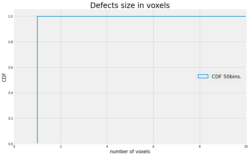
A continous random variable $X$ can take infinite possible variables.

Lets take as an example this list of defects extracted from a Ti6242 specimen manufactured via PBF-SLM.

We will start by examining the number of voxels occupied by each defect

#read the data
Mct = pd.read_csv('../Rep/defects.csv')

Mct.head()

	Radius [mm]	Diameter [mm]	Center x [mm]	Center y [mm]	Center z [mm]	Volume [mm³]	Voxel	Surface [mm²]	Gap [mm]	Compactness	...	Pos. x [mm]	Pos. y [mm]	Pos. z [mm]	Projected size x [mm]	Projected size y [mm]	Projected size z [mm]	Label	Projected area (yz-plane) [mm²]	Projected area (xz-plane) [mm²]	Projected area (xy-plane) [mm²]
0	0.0777	0.1554	-0.8663	2.7036	1.4228	0.000329	689	0.0545	-0.0348	0.17	...	-0.8595	2.7104	1.4193	0.1446	0.1251	0.0782	53790	0.0060	0.0069	0.0104
1	0.0530	0.1060	-1.2693	2.6135	5.5475	0.000157	328	0.0269	-0.0023	0.25	...	-1.2557	2.6173	5.5553	0.1016	0.0938	0.0547	110251	0.0034	0.0037	0.0057
2	0.0533	0.1066	2.0900	1.0270	2.5693	0.000175	367	0.0291	0.1123	0.28	...	2.0908	1.0160	2.5733	0.0938	0.1094	0.0547	71125	0.0042	0.0037	0.0062
3	0.0669	0.1338	4.0175	-1.2388	-4.0353	0.000175	366	0.0314	0.0052	0.14	...	4.0243	-1.2188	-4.0315	0.0860	0.1290	0.0625	8224	0.0045	0.0038	0.0064
4	0.0474	0.0949	-0.5736	-0.0857	4.1112	0.000130	271	0.0237	0.1406	0.29	...	-0.5721	-0.0812	4.1130	0.0860	0.0938	0.0547	88338	0.0035	0.0032	0.0048

5 rows × 21 columns

print('description of the number of voxels per defect','\n',Mct.Voxel.describe())

description of the number of voxels per defect 
 count    112048.000000
mean          1.409842
std           6.288546
min           1.000000
25%           1.000000
50%           1.000000
75%           1.000000
max         689.000000
Name: Voxel, dtype: float64

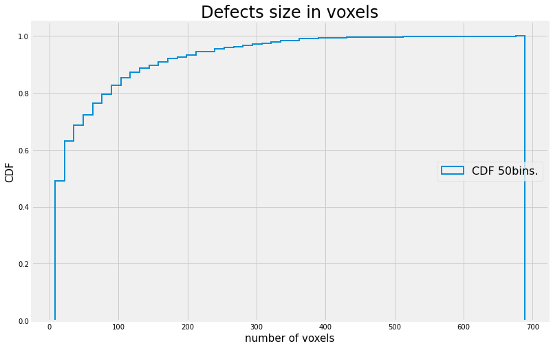
fig, ax = plt.subplots()
ax.hist(Mct.Voxel, bins=50, density=True, histtype='step', cumulative=1,
        label='CDF 50bins.', linewidth=2)

ax.grid(True)
ax.legend(loc='right',fontsize=16)
ax.set_title('Defects size in voxels',fontsize=24)
ax.set_xlabel('number of voxels',fontsize=15)
ax.set_ylabel('CDF',fontsize=15)
ax.set_xlim([0,10])

plt.show()

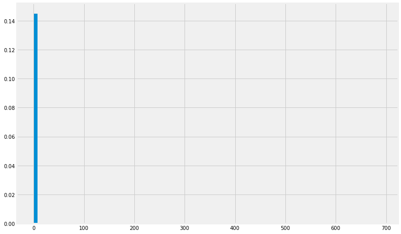
fig, axs = plt.subplots()

axs.hist(Mct.Voxel,bins=100, density=True);

#organize the headers
colnames=['Radius','Diameter','CenterX','CenterY','CenterZ','Volume','Voxel','Surface','Gap','Compactness',
'Sphericity','X','Y','Z','ProjectedX','ProjectedY','Projected','Label','ProjectedYZ','ProjectedXZ','ProjectedXY']
Mct.columns=colnames
#making things easier on the eye
Mct.set_index('Label')
Mct.sort_values(by='Label')
Mct['r']=Mct.apply(lambda row: np.sqrt(row.X*row.X+row.Y*row.Y),axis=1)
Mct.eval("theta = arctan2(X,Y)",  inplace=True)
Samp_vol =Mct.r.max() * Mct.r.max() *np.pi * (Mct.Z.max()-Mct.Z.min())
print('Estimated Sample Volume:', Samp_vol)
Mct.head()
Mctnew = Mct.drop(Mct[Mct.Voxel < 8].index).copy()

         

Estimated Sample Volume: 746.5442734136954

Mctnew.describe()

	Radius	Diameter	CenterX	CenterY	CenterZ	Volume	Voxel	Surface	Gap	Compactness	...	Z	ProjectedX	ProjectedY	Projected	Label	ProjectedYZ	ProjectedXZ	ProjectedXY	r	theta
count	415.000000	415.000000	415.000000	415.000000	415.000000	415.000000	415.000000	415.000000	415.000000	415.000000	...	415.000000	415.000000	415.000000	415.000000	415.000000	415.000000	415.000000	415.000000	415.000000	415.000000
mean	0.027697	0.055395	0.067099	0.819863	0.064835	0.000028	58.959036	0.008039	0.007397	0.225398	...	0.064916	0.048505	0.046791	0.033359	47885.212048	0.001193	0.001211	0.001430	2.789063	-0.038965
std	0.012050	0.024103	2.049289	1.988997	3.597330	0.000041	85.371118	0.007972	0.066483	0.094740	...	3.597026	0.022298	0.023096	0.013123	35446.875682	0.001038	0.001021	0.001448	1.016491	1.537667
min	0.012400	0.024700	-4.281100	-3.735600	-6.052800	0.000004	8.000000	0.001700	-0.039700	0.050000	...	-6.048900	0.015600	0.011700	0.007800	1.000000	0.000200	0.000200	0.000100	0.067113	-3.121345
25%	0.017500	0.035000	-1.518150	-0.916000	-2.698800	0.000005	11.000000	0.002400	-0.015700	0.150000	...	-2.698650	0.031300	0.027400	0.023500	17948.000000	0.000500	0.000500	0.000400	2.143471	-0.959730
50%	0.024100	0.048200	-0.033500	1.129900	0.243600	0.000010	22.000000	0.004300	-0.006700	0.200000	...	0.239500	0.043000	0.039100	0.031300	51432.000000	0.000700	0.000800	0.000800	2.871200	-0.068222
75%	0.037200	0.074400	1.824800	2.590750	2.791850	0.000034	72.000000	0.011600	0.001250	0.280000	...	2.794950	0.064450	0.062500	0.039100	71367.000000	0.001600	0.001600	0.002050	3.626132	0.904677
max	0.077700	0.155400	4.265800	4.336400	6.038300	0.000329	689.000000	0.054500	0.593100	0.530000	...	6.046100	0.144600	0.129000	0.093800	111991.000000	0.006600	0.006900	0.010400	4.405642	3.133515

8 rows × 23 columns

fig, ax = plt.subplots()
ax.hist(Mctnew.Voxel, bins=50, density=True, histtype='step', cumulative=1,
        label='CDF 50bins.', linewidth=2)

ax.grid(True)
ax.legend(loc='right',fontsize=16)
ax.set_title('Defects size in voxels',fontsize=24)
ax.set_xlabel('number of voxels',fontsize=15)
ax.set_ylabel('CDF',fontsize=15)


plt.show()

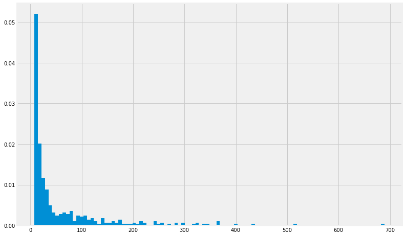
fig, axs = plt.subplots()

axs.hist(Mctnew.Voxel,bins=100, density=True);

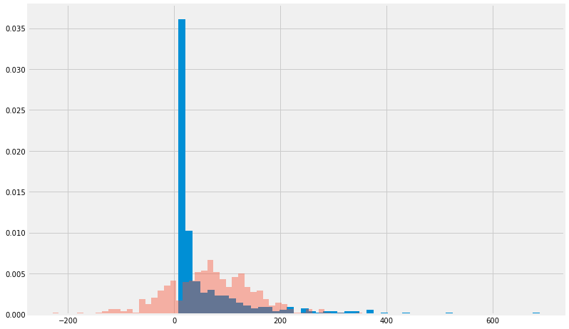
Now, this data doesnt seem to be following a normal distribution doesnt it?

Lets see what a normal distribution with the same mean and std woul look like:

from scipy.stats import norm
mu = Mctnew.Voxel.mean()
Var = np.power(Mctnew.Voxel.std(),2)
sigma = Mctnew.Voxel.std()
Vox = norm(mu,sigma)
fig, axs = plt.subplots()

axs.hist(Mctnew.Voxel,bins=50, density=True,label='experimental data');
axs.hist(Vox.rvs(415),bins=50, density=True,alpha=0.4, label='Normal distribution');

Here is the catch

We usually assume that our random variable is distributed in a normal distribution.

It has some advantages since it allows us to use $s$ in an intuitive manner and state that:

$~68\%$ of the data lies between $\bar{x} \pm s$
$~95\%$ of the data lies between $\bar{x} \pm 2s$
$~99.7\%$ of the data lies between $\bar{x} \pm 3s$
$3.4 X 10^{-5}$ of the data lies outside $\bar{x} \pm 6s$ (the six-sigma methodology)

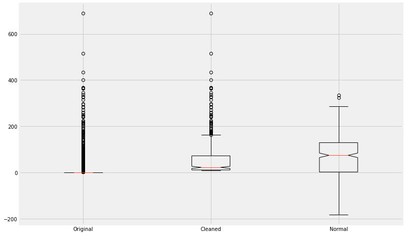
data=[Mct.Voxel, Mctnew.Voxel,Vox.rvs(415)]
plt.boxplot(data,notch=True);
plt.xticks([1,2,3],['Original','Cleaned','Normal'])

([<matplotlib.axis.XTick at 0x1986267aec8>,
  <matplotlib.axis.XTick at 0x19862411f08>,
  <matplotlib.axis.XTick at 0x19864ae6408>],
 [Text(1, 0, 'Original'), Text(2, 0, 'Cleaned'), Text(3, 0, 'Normal')])

Let us ignore the experimental data for a while and focus on the synthetic one.

fig, ax = plt.subplots()
SDefects = Vox.rvs(1000)
SDefects=SDefects-SDefects.min()
ax.hist(SDefects,bins='auto', density=False, histtype='step', cumulative=1,
        label='CDF', linewidth=2)
ax.hist(SDefects,bins='auto', density=False, cumulative=0,
        label='pdf', linewidth=2)
ax.grid(True)
ax.legend(loc='right',fontsize=16)
ax.set_title('Defects size in voxels',fontsize=24)
ax.set_xlabel('number of voxels',fontsize=15)
ax.set_ylabel('counts',fontsize=15)


plt.show()

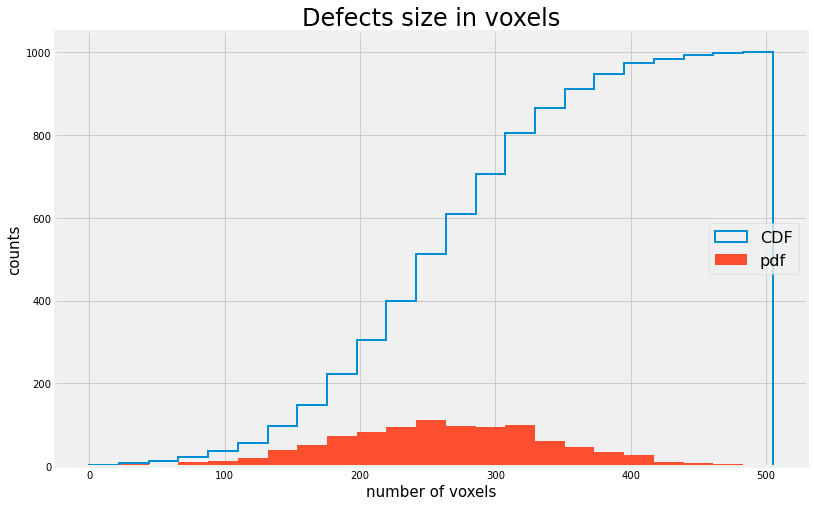
If we trust the algorithm we used to generate the defects data than the cruves above should represent a Normal ditribution

But how can we test that?

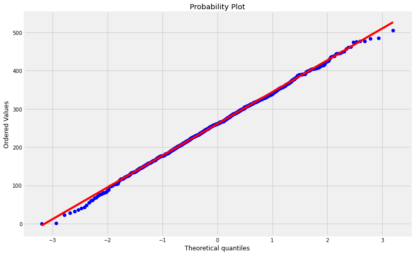
Assuming that the theoretical and actual probabilities are the same, we can rely on a simple and visual method to suppor our assumption:

Quantile-Quantile plot

The quantiles of each distribution should align with the other to form a straight line:

from scipy import stats

QQp=stats.probplot

QQp(SDefects,plot=plt);

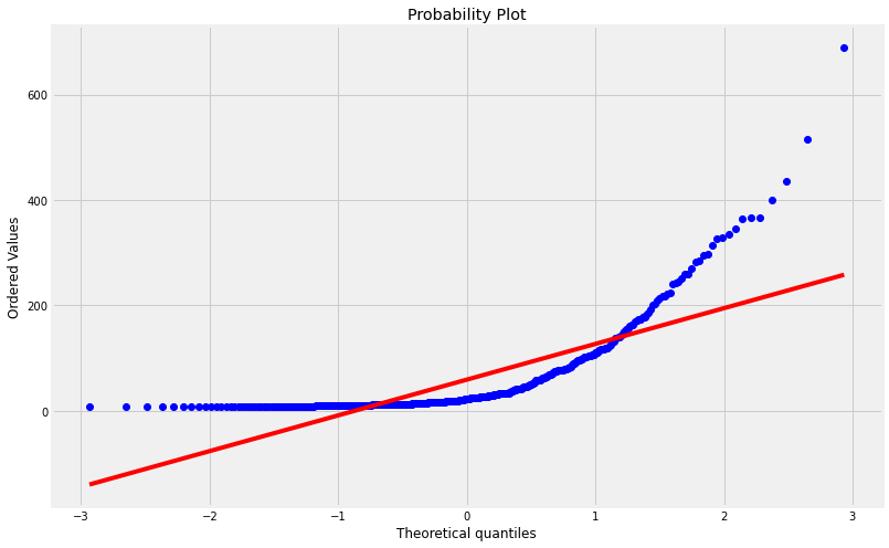
We can do the same for the experimental data in case we are not convinced it is not following a normal distribution:

QQp(Mctnew.Voxel,plot=plt);

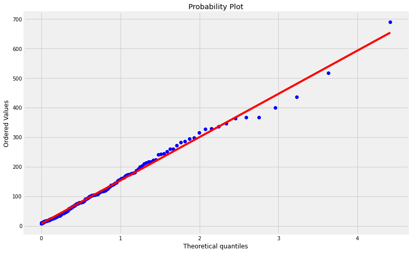
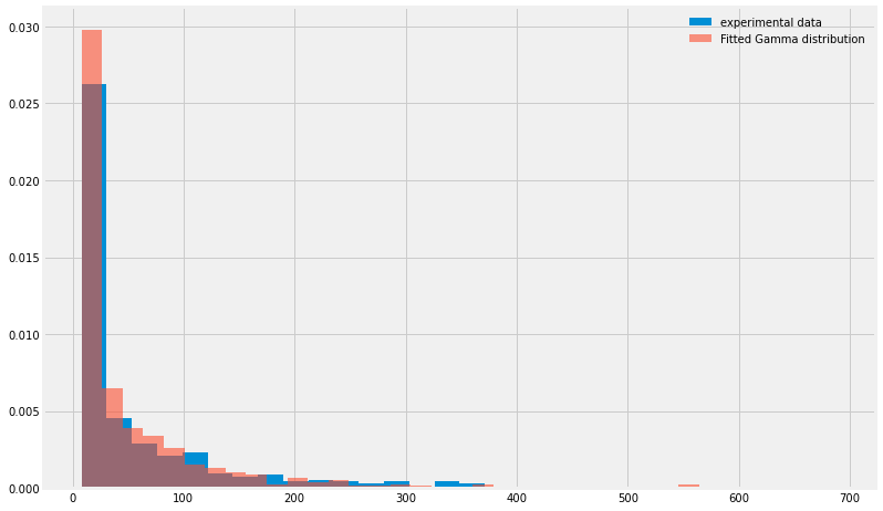
Or, if we try some other probability function, Lt’s take gamma for example:

a,b,c= stats.gamma.fit(Mctnew.Voxel)
G=stats.gamma(a, b,c);
GamProb = G.rvs(size=415);
x=np.linspace(G.ppf(0.01),G.ppf(0.99), 100)
GPDF = G.pdf(x)
QQp(Mctnew.Voxel,plot=plt ,dist=stats.gamma(a));

G=stats.gamma(a,b,c);
GamProb = G.rvs(size=415);
x=np.linspace(G.ppf(0.01),G.ppf(0.99), 100)
GPDF = G.pdf(x)

fig, axs = plt.subplots()

axs.hist(Mctnew.Voxel,bins=30, density=True,label='experimental data');
axs.hist(GamProb,bins=30,alpha=0.6,density=True,label='Fitted Gamma distribution');
axs.legend(loc='best', frameon=False)

plt.show()

16.1.5. Some common distributions¶

16.1.5.1. Normal distribution¶

We already met the normal distribution (Gaussian) which is commonly observed in many scenarios. This distribution is characterized by two parameters: $\mu$ - mean (center) and $\sigma$ - standard deviation (spread)

A random variable $X$ with a normal distribution is written as:

$X ∼ N(\mu,\sigma)$

and

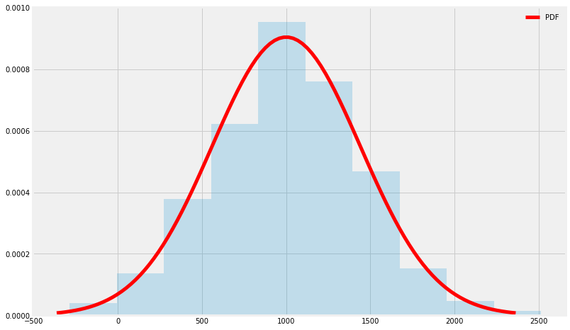
\[ f(x) = \frac{1}{\sigma \sqrt{2\pi}}\exp \left [ -\frac{1}{2}\left ( \frac{x-\mu}{\sigma} \right ) ^2 \right ] \]

Assumin $X$ is the number of cycles for failure in a fatigue test, and is characterized by $(\mu=21,\sigma=15)$

a=stats.norm(1000,21**2)

fig, ax = plt.subplots(1, 1)
x = np.linspace(a.ppf(0.001),
                a.ppf(0.999), 100)
ax.plot(x, a.pdf(x),
       'r-', lw=5, label='PDF')
       
CF = a.rvs(1000)
ax.hist(CF, density=True, histtype='stepfilled', alpha=0.2)
ax.legend(loc='best', frameon=False)
plt.show()

we can ask questions such as:

What is the probability of not failing after 100 cycles?

$P(X \gt 100) = 1-P(X \le 100) = 1-F(100) = 1- \int_{-\infty}^100 \frac{1}{21\sqrt{2 \pi}} \exp \left [ -\frac{1}{2}\left ( \frac{x-100}{21} \right ) ^2 \right ] $

print(1-a.cdf(10))

0.9876126580021647

What is the number of cycles for which we have less than a $0.1$ probability of failure?

print(a.ppf(0.1))

434.8357595948312

I assume you all remember that we can standarize the normal distribution such that :

$Z = \frac{X-\mu}{\sigma}$

and obtain $Z~N(0,1)$

What does the follwoing tell us?

print(a.cdf(1100) - a.cdf(900) )

0.17938758566989427

16.1.5.2. Exponential distribution¶

Recall the Poisson distribution we discussed in the context of discrete variables.

In that case we can state that $X$ is the number of failures in a week $(\lambda)$.

A continous description can be formulated as the time until failure $T_x$.

and the PDF & CDF of $t_x$ are given by :

\[\begin{split} F(t_x) =1- \exp ^{-\lambda t_x} \\ \\ \ \ \\ f(t_x)= \lambda\exp ^{-\lambda t_x} \end{split}\]

We will often use $\theta = \frac{1}{\lambda}$ such that $\theta$ will characterise the mean time until the first failure.

and now, (going back to $x$ fr simplicity)

\[ f(x) = \frac{1}{\theta} \exp \left [ \frac{-x}{\theta} \right ] \]

and :

\[ \mu = \theta \ \ ; \ \ \sigma = \theta \]

So, if a failure occur at a mean rate of $49$ cars a week and we can consider it as a Poisson process, what is the probability we will habe more than a day between failures?

$\lambda = 49/7 = 7$ cars a day and $\theta = \frac{1}{7}$ $\Rightarrow$ $f(t_x) = 7\exp (-7 t_x)$

$P(t_x>1) = \exp(-7*1) = 0.0009$

def Plot_exp(loc,scale):
    E=stats.expon(loc,scale)
    x = np.linspace(E.ppf(0.001),
                E.ppf(0.999), 100)
    CF = E.rvs(1000)
    return x,E.pdf(x),CF

    
fig, ax = plt.subplots(1, 1)
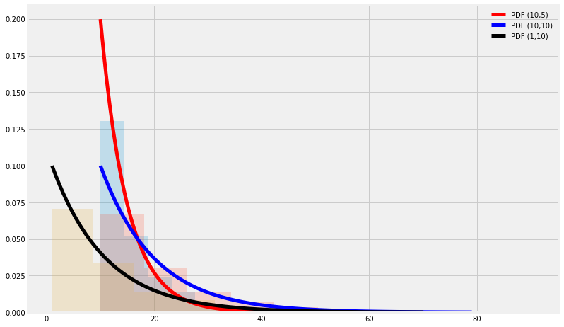
x,y,CF = Plot_exp(10,5)
ax.plot(x, y,'r-', lw=5, label='PDF (10,5)')
ax.hist(CF, density=True, histtype='stepfilled', alpha=0.2)

x,y,CF = Plot_exp(10,10)
ax.plot(x, y,'b-', lw=5, label='PDF (10,10)')
ax.hist(CF, density=True, histtype='stepfilled', alpha=0.2)

x,y,CF = Plot_exp(1,10)
ax.plot(x, y,'k-', lw=5, label='PDF (1,10)')
ax.hist(CF, density=True, histtype='stepfilled', alpha=0.2)

ax.legend(loc='best', frameon=False)
plt.show()

16.1.5.3. Exponential distribution $\to$ Gamma distribution¶

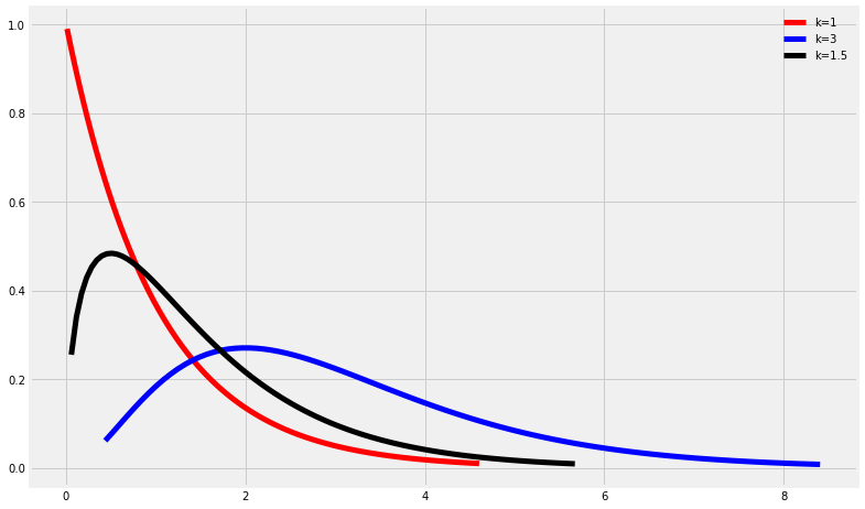
Now lets assume we wish to ask how much time we need to wait untile three cars break down.

the $F$ (cdf) of the expoential distribution told us when the next event will happen. Looking for the $n^{th}$ event is similar to :

$F(t_x) = 1-\sum_{k=0}^{n-1} \frac{(\lambda t_x)^k\exp (-\lambda t_x)}{k!}$

After some simple manipulation, we can show that $f(t_x) = F`(t_x)$ is given by for integer $k$ values :

\[ f(t_x) = \frac{t_x^{k-1}}{(k-1)!\theta^k}\exp(-\frac{t_x }{\theta}) \]

and

\[\begin{split} f(t_x) = \frac{t_x^{k-1}}{\Gamma(k)\theta^k}\exp(-\frac{t_x }{\theta}) \\ \\ \ \ \\ \Gamma(k) = \int_0^{\infty}y^{k-1}\exp(-y)dy \end{split}\]

otherwise.

the mean is given by $\mu = k\theta$ and the variance $\sigma^2$ is calculated from $\sigma = \sqrt{k}\theta$

def get_gam(a):
    x = np.linspace(stats.gamma.ppf(0.01, a),
                stats.gamma.ppf(0.99, a), 100)
    y = stats.gamma(a)
    return(x,y)
                    

fig, ax = plt.subplots(1, 1)

x,y=get_gam(1)              
ax.plot(x, y.pdf(x),'r-', lw=5, label='k=1')

x,y=get_gam(3)              
ax.plot(x, y.pdf(x),'b-', lw=5, label='k=3')

x,y=get_gam(1.5)              
ax.plot(x, y.pdf(x),'k-', lw=5, label='k=1.5')

ax.legend(loc='best', frameon=False)
plt.show()

16.1.6. From Gamma $\to$ Chi-Square¶

If our continous random varible $X$ follow a gamma distribution with $\theta =2$ and $2k=r$ with $r$ being a positive integer :

\[ f(x) = \frac{x^{r/2-1}}{\Gamma(\frac{r}{2})2^{r/2}}\exp(-\frac{x }{2}) \]

We will refer to it as a

Chi-Square

distribution with $r$ dof.

since it follows the gamma distribution the mean a variance of the Chi-Square are given by :

\[ \mu=E[X] =r \ \ \text{ and } \quad \sigma^2 = 2r \]

def get_chi2(dof):
    x = np.linspace(stats.chi2.ppf(0.01, dof),stats.chi2.ppf(0.99, dof), 100)
    y = stats.gamma(dof)
    return(x,y)
                    

fig, ax = plt.subplots(1, 1)

x,y=get_chi2(1)              
ax.plot(x, y.pdf(x),'r-', lw=5, label='r=1')

x,y=get_chi2(4)              
ax.plot(x, y.pdf(x),'b-', lw=5, label='r=4')

x,y=get_chi2(7)               
ax.plot(x, y.pdf(x),'k-', lw=5, label='r=7')

ax.legend(loc='best', frameon=False)
plt.show()

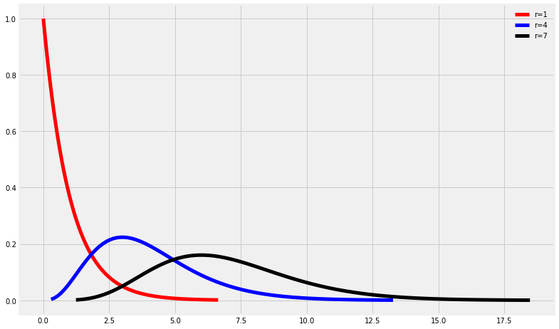
And if we are looking for the value of the random variable for which $P(X\le x) =0.75$ and we know that $r=7$ (black curve) we obtain:

print('x=',stats.chi2.ppf(0.75, 7))

x= 9.037147547908143

Similarly, the probability that our random variable is greater than 12.5 is :

print('x=',1-stats.chi2.cdf(12.5,10))

x= 0.25298532330929824

16.2. Statistical inference¶

When designing an experimental campaign we will, in many scenarios, aim at understanding a process or a phenomena or simply compare populations (e.g. different vendors)

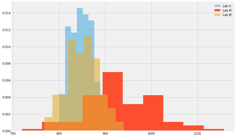
Let us examine the table below where the steady state pressure acting on a pressure vessel was measured at three different labs, 108 times for each lab:

PresMax = pd.read_csv('../rep/PressureMax.csv')
PresMax.describe()

	LocU	LocM	LocD
count	108.000000	108.000000	108.000000
mean	848.207680	932.301881	850.186908
std	24.866816	75.941999	35.216735
min	800.108198	718.892815	767.670008
25%	827.704051	888.556853	826.034777
50%	846.506359	924.015280	850.758706
75%	865.025943	984.351980	873.589351
max	927.304354	1157.256599	939.918922

fig, ax = plt.subplots(1, 1)
ax.hist(PresMax.LocU, density=True, histtype='stepfilled', alpha=0.4,label='Lab U')
ax.hist(PresMax.LocM, density=True, histtype='stepfilled', label='Lab M')
ax.hist(PresMax.LocD, density=True, histtype='stepfilled',alpha=0.6,label='Lab M')
ax.legend(loc='best', frameon=False)
plt.show()

16.2.1. Sampling variats¶

for $n$ which is not sufficiently large, we will use

\[ t=\frac{\sqrt{n} (\bar{x}-\mu)}{s} \]

in which $n$ is the DOF.

We will frequently be interested in the variations between the observable and not it mean. in those situations, we will resort to the Chi-Square dsitribution desribed above where:

\[ X^2 = \frac{s^2}{\sigma^2} (n-1) \]

is the variate of interest.

When comparing the variation between two processes or populations, we will often use the F-variate dfined as :

\[ F = \frac{s_1^2\sigma_2^2}{s_2^2 \sigma_1^2} \]

where the sample standard deviation $s$ of each popoulation/process contains the information regarding the number of samples.

16.2.2. Law(s) of large Numbers¶

Assume $X_i$ to be a set of measurements (independent random variables identically distributed) for which the expectation value is $E[X_i]=\mu$ and $\bar{X}=\frac{1}{n}\sum_i=1^nX_i$ , assuming a finite variance we can show that for sufficiently large $n$ we will obtain $\bar{X} \to \mu$
With $X$ being the same set of measurements as before, and $\mu = E[X_i] <\infty$ then $\bar{X} \to \mu$ for sufficiently large $n$.

$n$ can be estimated using $\sum\frac{\sigma_i^2}{i^2}$

16.2.3. Central limit theorem¶

Assumin that $\bar{X}$ is the mean of $X$ over $n$ measurements, for a sufficiently large $n$ we can show that

\[ Z_n=\frac{\sqrt{n}}{\sigma}\left ( \bar{X}-\mu \right ) \]

Approaches $N(0,1)$ as n increases.

Coming back to our example regarding the pressure data, looking at the sample mean of the U location we observe it to be $848.21$. But what does it tell us?

Using the standard error we can test how precise the estimator is.

16.2.4. Inference on a mean¶

writing the measured response as

\[ y_i = \mu + e_i \]

it means that $\bar{y}$ (the sample mean) is an estimator of the population mean $\mu$

Assuming that the errors $e_i$ are independent on eachother and normally distributed (as is often the case with random errors).

looking back on the t-distribution

\[ t = \frac{(\bar{y}-\mu)\sqrt{n}}{s} \]

Starting with :

\[ P[-t_{\alpha/2} < t < t_{\alpha/2}] = 1-\alpha \]

and doing some algebra we obtain :

\[ \bar{y} \pm t_{\alpha/2}s \]

which translates into the statement that:

we are $1-\alpha$ % sure that our confidience limits cover the unknown $\mu$ of the population mean.

looking at our examples we can find the 95% C.I for each location :

def print_CI(alpha, colName, dof):
    CIL = PresMax[colName].mean() -stats.t.ppf(1-alpha/2,df=107)*PresMax[colName].std()
    CIU = PresMax[colName].mean() -stats.t.ppf(alpha/2,df=107)*PresMax[colName].std()
    print ('For location',colName, 'the 95% CI is between ', CIL, 'and',CIU ,'and the sample mean is ',PresMax[colName].mean()) 
    

for colName in PresMax.columns:
    print_CI(0.05,colName,107)

For location LocU the 95% CI is between  798.9121173491465 and 897.5032419952981 and the sample mean is  848.2076796722223
For location LocM the 95% CI is between  781.7557248710715 and 1082.8480377178173 and the sample mean is  932.3018812944443
For location LocD the 95% CI is between  780.3738389715376 and 919.9999780136478 and the sample mean is  850.1869084925927

16.2.4.1. Hypothesis¶

Now lets test the hypothesis that the mean pressure in LocU is $825$

Our null hypothesis is

\[ H_0: \mu = 825 \]

And the alternative is

\[ H_a: \mu \ne 825 \]

using the t statistic we can formulate a decision rule:

Reject $ t>t_{\alpha/2} \ \ \text{or} \ \ t<t_{-\alpha/2}$

for LocU $t=0.745$ and $t_{\alpha/2} = 1.982$

We can estimate $n$ for a given $CI$ as:

\[ n = \left ( \frac{2 z_{\alpha /2} \sigma}{L} \right ) ^2 \]

How to compare the results from the different labs?

You were asked to conduct the experiment and report back if the new lab (LocM) is reliable

What will you say?

Welsch’s t-test

We can test if the results we obtained from the three independent labs represent the same mean (what is the meaning of population here?)

\[ t= \frac{\bar{X_1}-\bar{X_2}}{s_{w}} \]

\[ s_{w} = \sqrt{\frac{s_1^2}{n_1} + \frac{s_2^2}{n2}} \]

For LocU and LocD:

res = stats.ttest_ind(PresMax['LocU'],PresMax['LocD'], equal_var =False)
print('p-value is ',res.pvalue)

p-value is  0.6338258372488789

For LocU and LocM:

res = stats.ttest_ind(PresMax['LocU'],PresMax['LocM'], equal_var =False)
print('p-value is ',res.pvalue)

p-value is  3.9546450355445506e-20

16.2.5. Confidence intervals for the variance¶

The sample variance of $x$ is given by :

\[ \begin{align}\begin{aligned} s^2 = \frac{1}{n-1}\sum_i (x_i -\bar{x})^2 $$. \\since we alreday claimed that we can construct a variate $X$ which will follow a Chi-Square distribution :\end{aligned}\end{align} \]

X^2=(n-1) \left(\frac{s}{\sigma}\right )^2 $$

we can state that :

\[ P \left [ X^2_{1-\alpha/2} < (n-1) \left(\frac{s}{\sigma}\right )^2 < X^2_{\alpha/2} \right ]=1-\alpha \]

which will lead to

\[ P \left [ \frac{(n-1)s^2}{X^2_{\alpha/2}} < \sigma^2 < \frac{(n-1) s^2}{X^2_{1-\alpha/2}}\right ]=1-\alpha \]

and thus we now have a way of declaring the CI over $\sigma^2$ with 100(1-\alpha)% :

\[ \sqrt{\frac{(n-1)s^2}{X^2_{\alpha/2}} }< \sigma < \sqrt{\frac{(n-1) s^2}{X^2_{1-\alpha/2}}} \]

The hypothesis below may be used to check if the variance in the measurments of lab LocU us $\sigma_0^2$

$H_0 : \sigma_{LocU} = \sigma_{0}$

$H_{alt} : \sigma_{LocU} \ne \sigma_{0}$

However, we need to take one more step so that we can test if the data from the three labs has the same variance:

Using the $F$ variate we defined before :

\[ \frac{s_1^2}{s_2^2F_{\alpha/2}} < \left( \frac{\sigma_1}{\sigma_2} \right )^2 <\frac{s_1^2}{s_2^2F_{1-\alpha/2}} \]

Note that we have considered all of our measurments to arise from the same population of pressure vessels, otherwise we would have taken a different route.

Question

Assume the maximum allowed pressure is 900MPa

How will you go about deciding should you use the current design for operational pressure vessels?

16.2.6. Linear regression¶

A linear regression model will assume the form of :

\[ y_i = a_0 +a_1x_i + e_i \]

where $x_i$ can be alinear or non-linear functn of another predictor (you will find that $x=ln(z)$ is bein used quite often).

and is based on the assumptions that :

The $y$ is indeed dependent on $x$ in a linear manner (or it is a good approximation) in the range of interest
$x$ is measured withot (?) an error.
$e_i ~N(0,\sigma)$ with a constant variance.

16.3. To be continued¶

16.3.1. What to do when we have two variabales?¶

16.3.1.1. Covariance and Correlation¶

\[\begin{split} \text{Cov}(X,Y) = E[(X-\mu_x)(Y-\mu_y)] = \int \int (x-\mu_x)(y-\mu_y)f(x,y)dxdy =E[XY]-\mu_X\mu_Y =\sigma_{XY} \\ \\ \ \ \\ \text{Corr}(X,Y) = \frac{\sigma_{XY}}{\sigma_X \sigma_Y} \end{split}\]

Question

What can you tell me about $\text{Corr}(X,Y)$ ?

16.3.1.2. Joint probability ($X,Y \to $random variables)¶

The join probability density is given by :

\[ P(X,Y) = \int \int f(x,y)dxdy \]

So, lets think of it as an area measure.

Now, it simple to find things like $P(X<10,10<Y<50)$ or $P(X>Y)$ right?

We can define the marginal pdf of each variable following

\[ f_X(x) = \int f(x,y)dy \]

and their expectaction value :

\[ E[X]=\int \int xf(x,y)dxdy \]

we can even use $f_X(x),f_Y(y)$ to check if two variables are depndent or not by asking :

\[ f(x,y)=f_X(x)f_Y(y) ??? \]

16.3.1.3. Conditional probability¶

What is the probability of X for Y=y?

\[ h(x|y)=\frac{f(x,y)}{f_X(x)} \]

\[ E[X|y]=\int xh(x|y)dy \]

\[ \text{Var}(X|y) = E[X^2|y]-[E(X|y)]^2 \]

For a normal distribution and for a linear expectation value of $X$ given $y$ in which the conditional variance does not depend on the value of $x$ this translate into:

\[ (X|Y=y)~N \left ( \mu_X + \rho\frac{\sigma_Y}{\sigma_X}(Y-\mu_Y) \ \ , \ \ \sigma_X^2 (1-\rho^2) \right ) \]

When both $X$ and $Y$ are normally distributed we can write the joint probability density function as:

\[\begin{split} f(x,y)=\frac{1}{2\pi \sigma_X \sigma_Y \sqrt{1-\rho}}\exp \left ( -\frac{1}{2}q(x,y) \right ) \\ \\ \ \ \\ q(x,y) = \frac{1}{1-\rho^2} \left [ \left( \frac{X-\mu_X}{\sigma_X} \right )^2 + \left( \frac{Y-\mu_Y}{\sigma_Y} \right )^2 - 2 \rho \frac{X-\mu_X}{\sigma_X}\frac{Y-\mu_Y}{\sigma_Y} \right ] \end{split}\]

ME034044notes

Analysis of Experimental Measurments

Contents

16. Analysis of Experimental Measurments¶

16.1. Probability¶

16.1.1. Discrete variables¶

16.1.1.1. Not all distributions are born the same¶

16.1.2. The expectation value - characterizing the central tendency¶

16.1.3. The variance - characterizing the spread¶

16.1.4. Continous variables¶

16.1.5. Some common distributions¶

16.1.5.1. Normal distribution¶

16.1.5.2. Exponential distribution¶

16.1.5.3. Exponential distribution \(\to\) Gamma distribution¶

16.1.6. From Gamma \(\to\) Chi-Square¶

16.2. Statistical inference¶

16.2.1. Sampling variats¶

16.2.2. Law(s) of large Numbers¶

16.2.3. Central limit theorem¶

16.2.4. Inference on a mean¶

16.2.4.1. Hypothesis¶

16.2.5. Confidence intervals for the variance¶

16.2.6. Linear regression¶

16.3. To be continued¶

16.3.1. What to do when we have two variabales?¶

16.3.1.1. Covariance and Correlation¶

16.3.1.2. Joint probability (\(X,Y \to \)random variables)¶

16.3.1.3. Conditional probability¶

16.4. To be continued¶