Uncertainties and Error Propagation
4. Uncertainties and Error Propagation
In the previous week we have discussed the various sources of errors. It is important that we distinguish between the concepts of error and uncertainty.
Once all of the errors in our measurement were accounted for (e.g. bias, noises etc.), we are still uncertain as to the true value of the measured variable.
As you recall, we have discussed two types of errors: systematic errors and random errors.
Systematics errors in the form o bias for example, can be accounted for using proper calibration. Other systematic errors may be the results of system degradation, and thus will not appear constant (hence the recommendation for routine calibration). Another type of systematic errors (which you of course will never have) is a poor design of the experimental system.
Offset
Scaling/calibration issues
drifting
Can you come up with examples of potential pitfalls leading to systematic errors?
Random errors, as suggested by their name, are hard to predict and identify. In many cases, (not always!) random errors will have an expectation value (\(E(X)\)) of \(0\) and thus we assume (or hope) that repeating the measurement enough times will minimize the random errors.
How many repetitions should be made?
The term uncertainty reflects the fact that we simply dont know the true value of the variable we are measuring. Even after we have accounted for all the systematic errors, there still may be some we have missed. Our random errors may be dependent on many unforeseen variables or distributed in a different way than we assume, etc.
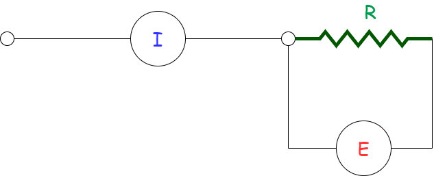
Lets consider a simple case, where we simply try to calculate the \(\color{red}{\text{voltage}}\) based on an input \(\color{blue}{\text{current}}\) and known \(\color{green}{\text{resistance}}\) using:
Unfortunately the know \(\color{blue}{\text{current}}\) is only known up to \(\color{blue}{0.1mA}\) and the resistor we use is characterized by \(\color{green}{R=5 \ \ Ohm \pm 0.01 }\)
Assuming we measured a \(\color{blue}{\text{current}}\) of \(\color{blue}{5A}\) we could claim that the nominal result is \(\color{red}{V=25 V}\)
However, taking the worst possible cases will lead to:
As you may remember, we can propagate the uncertainty using:
Note
The above expression is a linear approximation. TheWe will go over the associated assumption and other methods for uncertainty estimation later in the course.
which in our case will lead to :
It doesn’t seem like a huge change but try playing with the measurement value and see the effect…
The uncertainty propagation concept can aid us in choosing the proper measurement tool. Assume you assemble the following circuit using a resistor with \(\color{green}{R=10 \ \ Ohm \pm 1\% }\).
You can calculate the power dissipation using either:
Given that :
Which measurement will you choose?
To answer that we can use the equation for \(\sigma\) and see that for (1) the uncertainty is \(2.236 \% \) while for (2) it reduces for \( 1.414 \% \).
‘’’{admonition} Easy to use uncertainty calculators
To be continued…