8. Dynamic Systems - Part 2¶

import numpy as np

import matplotlib.pyplot as plt
from ipywidgets import widgets, interact
from IPython import display

Reminder from last lecture:

An \(N^{th}\) order system with an output signal \(y(t)\), when subjected to a general input signal represented by the forcing signal \(F(t)\) is given by:

\[\begin{split} a_n \frac{d^n y}{dt^n}+a_{n-1} \frac{d^{n-1} y}{dt^{n-1}}+\cdot \cdot \cdot +a_{1} \frac{d y}{dt} + a_0 y= F(t) \\ F(t) = b_m \frac{d^m x}{dt^m}+b_{m-1} \frac{d^{m-1} x}{dt^{m-1}}+\cdot \cdot \cdot +b_{1} \frac{d x}{dt} + b_0 x \quad m \leq n \end{split}\]

and the coefficients \(a_i\) and \(b_j\) are a representation of physical parameters of the measuring system

8.1. 2\(^{nd}\) order systems¶

\[ a_2 \frac{d^2y(t)}{dt^2} + a_1 \frac{dy(t)}{dt} + a_0 y(t) = F(t) \]

Normalizing the equation by \(a_2\) will lead to :

\[ \frac{1}{{\color{blue}{\omega ^2}}}\frac{d^2y(t)}{dt^2} + \frac{2{\color{red}{\xi}}}{{\color{blue}{\omega}}} \frac{dy(t)}{dt} + y(t) ={\color{green}{K}} F(t) \]

With :

\[\begin{split} \frac{1}{{\color{blue}{\omega^2}}} = \frac{a_2}{a_0} = {\color{blue}{\tau_s}}^2 \\ \frac{2{\color{red}{\xi}}}{{\color{blue}{\omega}}} = \frac{a_1}{a_0} \\ {\color{green}{K}} = \frac{1}{a_0} \end{split}\]

In the above equation the three constnat are:

\(\color{green}{K}\) - gain parameter (similar to the linear sensitivity from before)
\(\color{red}{\xi}\) - damping parameter
\(\color{blue}{\tau_S}\) - characteristic time

8.2. Load cell as a \(2^{nd}\) order system¶

Many load cells rely on the elastic deformation of a structure with a known compliance. By measuring the deformation (using e.g. strain gauges) and relying on the compliance the force is extracted (think of a simple spring, it’s not that different as a 0 order approximation).

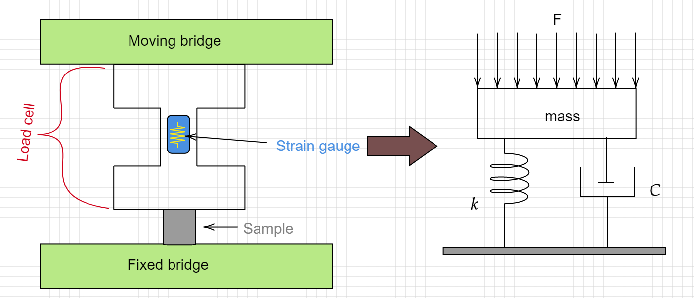
The applied force is being opposed by two components, a linear spring with a spring constant \(\color{blue}{k}\) and a dashpot characterized by \(\color{red}{C}\)

We can model this system using the following set of equations:

\[ {\color{blue}{m}}\frac{dx_m^2}{dt^2} = -{\color{red}{C}} \frac{dx_m}{dt} -{\color{green}{k}}x_m + F \]

From the above we easily obtain that :

\[\begin{split} {\color{red}{\xi}} = \frac{{\color{red}{C}}}{2 \sqrt{{\color{green}{k}}{\color{blue}{m}}}} \\ {\color{blue}{\omega_0}} = \sqrt{\frac{\color{green}{k}}{\color{blue}{m}}} \end{split}\]

Note

The applied force \(F\) is not the same as the measured force \(F_m\) due to the damping of the system. Can you estimate under what conditions \(F=F_m\) ?

Rearranging the \(2^{nd}\) order system, and adding a time delay parameter to the input function (remember the dashpot) we can write our equation as

\[ {\color{blue}{\tau_s}}^2 \frac{d^2y}{dt^2} + 2{\color{red}{\xi}}{\color{blue}{\tau_s}}\frac{dy}{dt} + y = \color{green}{K}F(t-\theta) \]

Which we will solve numerically using scipy.integrate.odeint

from scipy.integrate import odeint
K = 1.2
tau = 0.2
zeta = 0.1
theta = 0.0
du = 1.0
yInf = K*du
def SOS_ODE(x,t):
    y = x[0]
    dydt = x[1]
    dy2dt2 = (-2.0*zeta*tau*dydt - y + K*du)/tau**2
    return [dydt,dy2dt2]

t = np.arange(0,14,0.010)
x = odeint(SOS_ODE,[0,0],t)
y = x[:,0]
yInf = K*du


fig, ax = plt.subplots(figsize=(18, 8),sharex=True, sharey=True)
ax.plot(t,y,'r-',linewidth=2,label='ODE Integrator')
ax.plot([0,max(t)],[yInf,yInf],'k--')
ax.plot([0,max(t)],[1.1*yInf,1.1*yInf],'b--')
ax.plot([0,max(t)],[0.9*yInf,0.9*yInf],'b--')
ax.set_xlabel('Time', fontsize=14)
ax.set_ylabel('y(t)', fontsize=14)

---------------------------------------------------------------------------
ModuleNotFoundError                       Traceback (most recent call last)
Input In [2], in <cell line: 1>()
----> 1 from scipy.integrate import odeint
      2 K = 1.2
      3 tau = 0.2

ModuleNotFoundError: No module named 'scipy'

solving for a sin() input

import scipy.signal as sg
#K = 1.5
#tau = 0.8
#zeta = 0.4
theta = 0.0
#here we will use the transfer function
%matplotlib inline
plt.rcParams['figure.figsize'] = [20, 10]
def second_order_w_sin(tau,K,xi,Omega):
    Tvec = np.arange(0.0, 20*np.pi/Omega, 0.05)
    num = [K]
    den = [np.power(tau,2),2*xi*tau,1]
    SoS = sg.TransferFunction(num,den)
    Ft = np.sin(Omega*Tvec)
    Tout, sinRes, xout = sg.lsim(SoS, Ft, Tvec)
    fig, ax = plt.subplots(1, 1, figsize=(18, 8),sharex=False, sharey=False)
    ax.plot(Tvec*Omega/(2*np.pi), sinRes,label='system response',color='blue')
    ax.plot(Tvec*Omega/(2*np.pi), Ft,label='system input',color='green')
    ax.set_xlabel('Normalized time')
    ax.set_title(r'response to s sin input $\omega \tau$ = %f'%(Omega*tau), fontsize=14)
    ax.legend()


# Simulate tau * dy/dt = -y + F(omega)

interact(second_order_w_sin, tau = (0.1,5,0.1), K= (0.0,2,0.1), xi= (0.0,1,0.05), Omega = (0.1,5,0.1))

<function __main__.second_order_w_sin(tau, K, xi, Omega)>

So….

What will happen if we have a mass with negligible accelaration but finite velocity?

we can write the dynamic error as

\[ e = F_m - F = kx_m -F \approx -C\dot{x}_m \]

a rising force, will lead to a positive \(\dot{x}_m\) resulting in a negative \(e\) and vice versa.

In other words, the damping is behind the measured hysteresis

Let’s try to sum it up :

Sensor’s property	System behavior
\(\big\Downarrow\) \(k\)	High sensitivity
\(\big\Downarrow\) \(\xi\),\(\to\) \(\big\Downarrow\) \(C\)	Low hysteresis
\(\big\Downarrow\) m, \(\big\Downarrow\) \(\xi\), \(\big\Uparrow\) \(\omega_0\), \(\big\Downarrow\) \(k\)	Minimize the phase shift over a large frequency range
\(\big\Downarrow\) m, \(\big\Downarrow\) \(\xi\), \(\big\Uparrow\) \(\omega_0\), \(\big\Downarrow\) \(k\)	Amplitude ratio approaching 1 over a large frequency range
\(\xi\) sufficiently large (or not too small)	Decrease “ringing” due to step input

ME034044notes

Dynamic Systems - Part 2

Contents

8. Dynamic Systems - Part 2¶

8.1. 2\(^{nd}\) order systems¶

8.2. Load cell as a \(2^{nd}\) order system¶