import sys, os
sys.path.insert(0, os.path.join(os.pardir, 'src'))

import sympy as sp
import numpy as np
import matplotlib.pyplot as plt
from IPython.display import Math, display, Markdown

from symbolic_fem_workbench import (
    build_bar_1d_local_problem,
    build_bar_1d_mass_matrix,
    LinearElement1D, local_trial_expansion, local_test_expansion,
    extract_coefficient_matrix,
    assemble_dense_matrix, assemble_dense_vector,
    apply_dirichlet_by_reduction, expand_reduced_solution,
)14 Time-Dependent FEM: Mass Matrix and Time Stepping
This notebook covers the semi-discrete FEM formulation for time-dependent problems. We build the consistent mass matrix \(M_e\) using the workbench, assemble it alongside the stiffness matrix \(K\), and solve using both implicit (backward Euler) and explicit (forward Euler) time-stepping schemes.
Learning objectives:
- Derive the element mass matrix \(M_e = \int \rho A \, N^T N \, dx\) symbolically.
- Understand the semi-discrete system \(M \ddot{a} + K a = F\) (or \(M \dot{a} + K a = F\) for parabolic problems).
- Compare lumped vs. consistent mass matrices.
- Implement backward Euler and forward Euler time stepping.
- Observe the CFL stability limit for explicit schemes.
14.1 1. Symbolic Mass Matrix Derivation
For a time-dependent heat equation \(\rho c \, \partial u / \partial t = \partial/\partial x(k \, \partial u / \partial x) + q\), the FEM semi-discretization yields:
\[M \dot{a} + K a = F\]
where \(M_{ij} = \int_0^L \rho c \, N_i \, N_j \, dx\) is the consistent mass matrix.
The workbench derives this symbolically for a two-node linear element:
mass = build_bar_1d_mass_matrix()

display(Markdown("**Element mass matrix $M_e$:**"))
display(Math(sp.latex(mass['Me'])))

display(Markdown(f"**Symbols:** L = {mass['L']}, rho = {mass['rho']}, A = {mass['A']}"))
Element mass matrix \(M_e\):
\(\displaystyle \left[\begin{matrix}\frac{A L \rho}{3} & \frac{A L \rho}{6}\\\frac{A L \rho}{6} & \frac{A L \rho}{3}\end{matrix}\right]\)
Symbols: L = L, rho = rho, A = A
14.1.1 Lumped Mass Matrix
A common simplification is the lumped mass matrix, obtained by summing each row of the consistent mass matrix and placing the result on the diagonal. This makes the mass matrix diagonal, which is critical for explicit time-stepping efficiency.
Me = mass['Me']
rho, A, L = mass['rho'], mass['A'], mass['L']

# Lumped mass: row-sum technique
Me_lumped = sp.diag(*[sum(Me.row(i)) for i in range(Me.rows)])

display(Markdown("**Consistent mass matrix:**"))
display(Math(sp.latex(Me)))

display(Markdown("**Lumped mass matrix (row-sum):**"))
display(Math(sp.latex(Me_lumped)))

display(Markdown(
    "Note: Both have the same total mass $\\rho A L$, but the lumped version "
    "distributes it equally to the two nodes."
))
Consistent mass matrix:
\(\displaystyle \left[\begin{matrix}\frac{A L \rho}{3} & \frac{A L \rho}{6}\\\frac{A L \rho}{6} & \frac{A L \rho}{3}\end{matrix}\right]\)
Lumped mass matrix (row-sum):
\(\displaystyle \left[\begin{matrix}\frac{A L \rho}{2} & 0\\0 & \frac{A L \rho}{2}\end{matrix}\right]\)
Note: Both have the same total mass \(\rho A L\), but the lumped version distributes it equally to the two nodes.
14.2 2. Also Retrieve the Stiffness Matrix and Load Vector
We need \(K_e\) and \(f_e\) for the full semi-discrete system.
bar = build_bar_1d_local_problem()

display(Markdown("**Element stiffness matrix $K_e$:**"))
display(Math(sp.latex(bar['Ke'])))

display(Markdown("**Element load vector $f_e$:**"))
display(Math(sp.latex(bar['fe'])))
Element stiffness matrix \(K_e\):
\(\displaystyle \left[\begin{matrix}\frac{A E}{L} & - \frac{A E}{L}\\- \frac{A E}{L} & \frac{A E}{L}\end{matrix}\right]\)
Element load vector \(f_e\):
\(\displaystyle \left[\begin{matrix}\frac{L q}{2}\\\frac{L q}{2}\end{matrix}\right]\)
14.3 3. Numerical Assembly: 1D Heat Equation
We solve the 1D transient heat equation on \([0, 1]\) with:
- \(k = 1\) (thermal conductivity), \(\rho c = 1\)
- \(q = 0\) (no source)
- BC: \(u(0,t) = 0\), \(u(1,t) = 0\)
- IC: \(u(x,0) = \sin(\pi x)\)
Exact solution: \(u(x,t) = \sin(\pi x) \, e^{-\pi^2 t}\)
# ---- Mesh and material parameters ----
n_elem = 10
L_total = 1.0
k_cond = 1.0   # conductivity (plays role of EA)
rho_c = 1.0     # rho * c  (plays role of rho*A)
h_e = L_total / n_elem
n_nodes = n_elem + 1
x_nodes = np.linspace(0, L_total, n_nodes)

# ---- Numerical element matrices ----
# Stiffness for pure diffusion: Ke = (k/h) * [[1, -1], [-1, 1]]
# We build this directly from the symbolic Ke (set q=0, P=0 for no source/traction)
Ke_sym = bar['Ke']
Ke_num = np.array(Ke_sym.subs({bar['E']: k_cond, bar['A']: 1, bar['L']: h_e, bar['q']: 0, bar['P']: 0})).astype(float)

# Mass: Me = (rho_c * h / 6) * [[2, 1], [1, 2]]
Me_num = np.array(Me.subs({rho: rho_c, A: 1, L: h_e})).astype(float)

# Lumped mass
Me_lumped_num = np.array(Me_lumped.subs({rho: rho_c, A: 1, L: h_e})).astype(float)

print(f"Element stiffness Ke:\n{Ke_num}")
print(f"\nConsistent mass Me:\n{Me_num}")
print(f"\nLumped mass Me_lumped:\n{Me_lumped_num}")
Element stiffness Ke:
[[ 10. -10.]
[-10. 10.]]
Consistent mass Me:
[[0.03333333 0.01666667]
[0.01666667 0.03333333]]
Lumped mass Me_lumped:
[[0.05 0. ]
[0. 0.05]]# ---- Global assembly ----
K_global = np.zeros((n_nodes, n_nodes))
M_global = np.zeros((n_nodes, n_nodes))
M_lumped_global = np.zeros((n_nodes, n_nodes))
connectivity = [[e, e+1] for e in range(n_elem)]
for conn in connectivity:
assemble_dense_matrix(K_global, Ke_num, conn)
assemble_dense_matrix(M_global, Me_num, conn)
assemble_dense_matrix(M_lumped_global, Me_lumped_num, conn)
print(f"Global K shape: {K_global.shape}")
print(f"Global M shape: {M_global.shape}")Global K shape: (11, 11)
Global M shape: (11, 11)14.4 4. Time Stepping: Backward Euler (Implicit)
The backward Euler scheme for \(M \dot{a} + K a = F\):
\[(M + \Delta t \, K) \, a^{n+1} = M \, a^n + \Delta t \, F^{n+1}\]
This is unconditionally stable (no CFL limit), but requires solving a linear system at each time step.
# ---- Backward Euler ----
dt = 0.005
T_final = 0.05
n_steps = int(T_final / dt)

# Initial condition: u(x,0) = sin(pi*x)
u_be = np.sin(np.pi * x_nodes).copy()

# Apply Dirichlet BCs: u(0)=0, u(1)=0 at all times
bc_dofs = [0, n_nodes - 1]
free_dofs = list(range(1, n_nodes - 1))

# Reduced system matrices (free DOFs only)
M_ff = M_global[np.ix_(free_dofs, free_dofs)]
K_ff = K_global[np.ix_(free_dofs, free_dofs)]

# Effective stiffness: A_eff = M + dt*K
A_eff = M_ff + dt * K_ff

# Store solutions for plotting
solutions_be = [u_be.copy()]
times = [0.0]

for step in range(n_steps):
    t_new = (step + 1) * dt
    rhs = M_ff @ u_be[free_dofs]  # F = 0 (no source)
    u_be[free_dofs] = np.linalg.solve(A_eff, rhs)
    # BCs remain zero
    solutions_be.append(u_be.copy())
    times.append(t_new)

print(f"Backward Euler: {n_steps} steps, dt = {dt}")
Backward Euler: 10 steps, dt = 0.00514.5 5. Time Stepping: Forward Euler (Explicit)
The forward Euler scheme:
\[M \, a^{n+1} = (M - \Delta t \, K) \, a^n + \Delta t \, F^n\]
With a lumped (diagonal) mass matrix, no system solve is needed — just a diagonal scaling. But there is a CFL stability limit: \(\Delta t < 2 / \lambda_{\max}\) where \(\lambda_{\max}\) is the largest eigenvalue of \(M^{-1} K\).
# ---- CFL stability analysis ----
M_lump_ff = M_lumped_global[np.ix_(free_dofs, free_dofs)]
M_lump_inv = np.diag(1.0 / np.diag(M_lump_ff))
eigenvalues = np.linalg.eigvalsh(M_lump_inv @ K_ff)
lambda_max = eigenvalues.max()
dt_crit = 2.0 / lambda_max

print(f"Largest eigenvalue of M_lump^{{-1}} K: {lambda_max:.4f}")
print(f"Critical time step (CFL): dt_crit = {dt_crit:.6f}")
print(f"Our dt = {dt} {'< dt_crit (STABLE)' if dt < dt_crit else '>= dt_crit (UNSTABLE!)'}")
Largest eigenvalue of M_lump^{-1} K: 390.2113
Critical time step (CFL): dt_crit = 0.005125
Our dt = 0.005 < dt_crit (STABLE)# ---- Forward Euler with lumped mass ----
dt_fe = min(dt, 0.9 * dt_crit) # stay below CFL
n_steps_fe = int(T_final / dt_fe)
u_fe = np.sin(np.pi * x_nodes).copy()
solutions_fe = [u_fe.copy()]
times_fe = [0.0]
M_lump_diag = np.diag(M_lump_ff)
for step in range(n_steps_fe):
t_new = (step + 1) * dt_fe
rhs = M_lump_ff @ u_fe[free_dofs] - dt_fe * (K_ff @ u_fe[free_dofs])
u_fe[free_dofs] = rhs / M_lump_diag # diagonal solve!
solutions_fe.append(u_fe.copy())
times_fe.append(t_new)
print(f"Forward Euler: {n_steps_fe} steps, dt = {dt_fe:.6f}")Forward Euler: 10 steps, dt = 0.00461314.6 6. Comparison with Exact Solution
def exact_solution(x, t):
    return np.sin(np.pi * x) * np.exp(-np.pi**2 * t)

fig, axes = plt.subplots(1, 3, figsize=(14, 4))

# Plot at select times
plot_times = [0, T_final/2, T_final]
x_fine = np.linspace(0, L_total, 200)

for ax, t_plot in zip(axes, plot_times):
    # Exact
    ax.plot(x_fine, exact_solution(x_fine, t_plot), 'k-', lw=2, label='Exact')

    # Backward Euler
    idx_be = min(range(len(times)), key=lambda i: abs(times[i] - t_plot))
    ax.plot(x_nodes, solutions_be[idx_be], 'bo-', ms=4, label='Backward Euler')

    # Forward Euler
    idx_fe = min(range(len(times_fe)), key=lambda i: abs(times_fe[i] - t_plot))
    ax.plot(x_nodes, solutions_fe[idx_fe], 'rs--', ms=4, label='Forward Euler')

    ax.set_title(f't = {t_plot:.3f}')
    ax.set_xlabel('x')
    ax.set_ylabel('u(x,t)')
    ax.legend(fontsize=8)
    ax.grid(True, alpha=0.3)

fig.suptitle('1D Transient Heat Equation: FEM Solutions vs Exact', fontsize=13)
plt.tight_layout()
plt.show()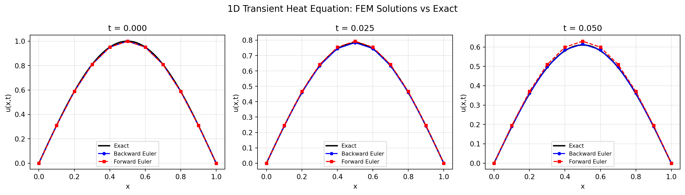
14.7 7. Demonstrating Instability
What happens if we use \(\Delta t > \Delta t_{\text{crit}}\) with the explicit scheme?
# ---- Unstable forward Euler ----
dt_unstable = 1.1 * dt_crit
u_unstable = np.sin(np.pi * x_nodes).copy()
n_steps_unstable = min(20, int(T_final / dt_unstable))  # limit steps to avoid overflow

max_vals = [np.max(np.abs(u_unstable))]

for step in range(n_steps_unstable):
    rhs = M_lump_ff @ u_unstable[free_dofs] - dt_unstable * (K_ff @ u_unstable[free_dofs])
    u_unstable[free_dofs] = rhs / M_lump_diag
    max_vals.append(np.max(np.abs(u_unstable)))
    if max_vals[-1] > 1e6:
        print(f"Blew up at step {step+1}!")
        break

fig, ax = plt.subplots(figsize=(8, 4))
ax.semilogy(range(len(max_vals)), max_vals, 'r-o', ms=4)
ax.set_xlabel('Time step')
ax.set_ylabel('max |u|')
ax.set_title(f'Forward Euler instability: dt = {dt_unstable:.6f} > dt_crit = {dt_crit:.6f}')
ax.grid(True, alpha=0.3)
plt.tight_layout()
plt.show()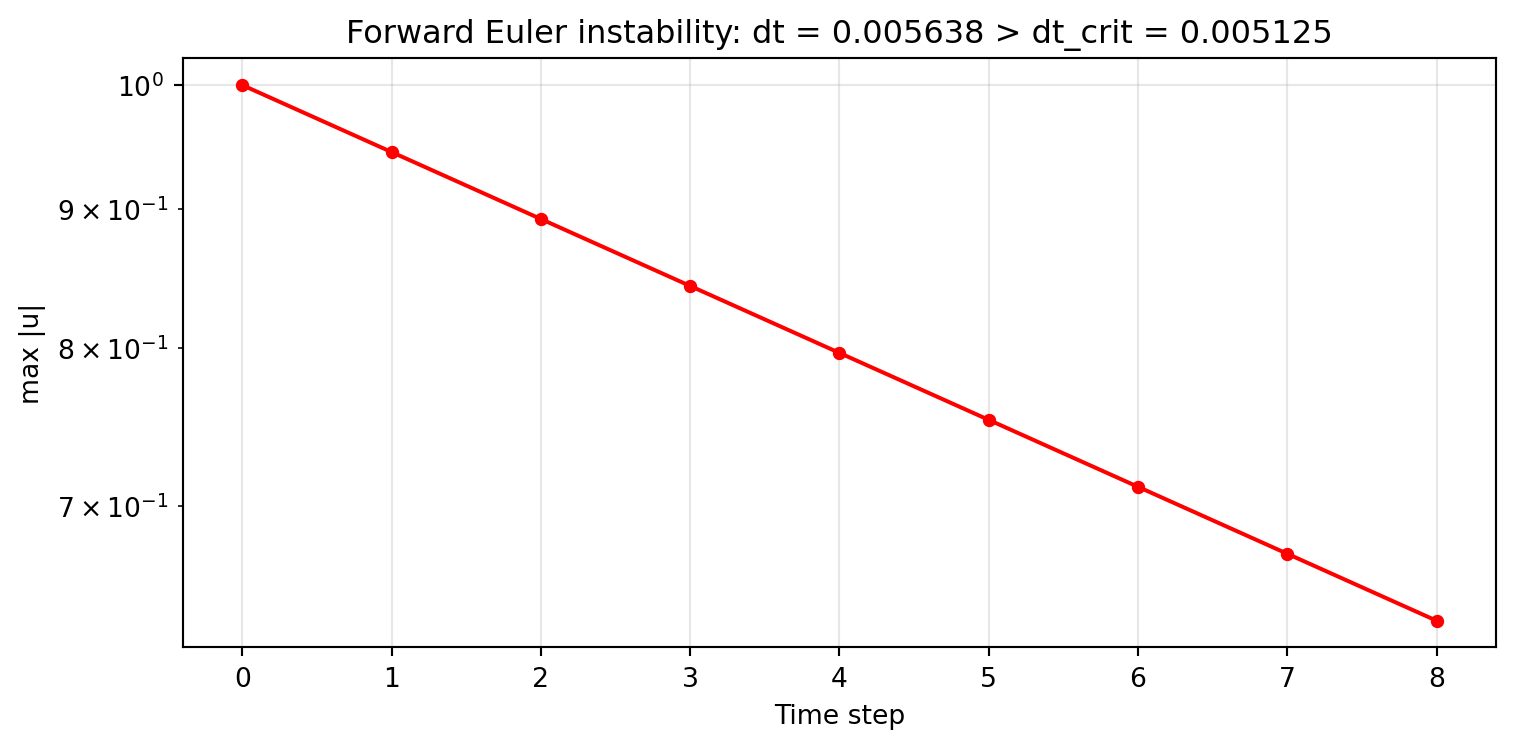
14.8 Summary
| Aspect | Backward Euler | Forward Euler (lumped M) |
|---|---|---|
| Stability | Unconditionally stable | \(\Delta t < 2/\lambda_{\max}\) |
| System solve per step | Yes (sparse LU or CG) | No (diagonal scaling) |
| Accuracy | \(O(\Delta t)\) | \(O(\Delta t)\) |
| Best for | Stiff problems, large \(\Delta t\) | Wave propagation, small \(\Delta t\) |
Key takeaway: The mass matrix is as fundamental as the stiffness matrix in FEM. The workbench derives it symbolically from the same shape functions used for \(K_e\).