8  Manual 2D Assembly: From Local Tensors to Global Solution

This notebook demonstrates the assembly process: combining element matrices and vectors into a global system, applying boundary conditions, and solving for the finite element solution. Assembly is fundamentally a topological operation—it depends only on node connectivity, not on the analytical properties of elements.

import sympy as sp
import numpy as np
import matplotlib.pyplot as plt
from IPython.display import Math, display
from symbolic_fem_workbench import (
    build_poisson_triangle_p1_local_problem,
    assemble_dense_matrix, assemble_dense_vector,
    apply_dirichlet_by_reduction, expand_reduced_solution,
)

8.1 Step 1: Get symbolic local tensors and convert to numerical

We retrieve the element stiffness matrix and load vector from the previous notebook and convert them to numerical functions via lambdify.

data = build_poisson_triangle_p1_local_problem()
geom = data["geometry"]

ke_fn = sp.lambdify(
    (geom.x1, geom.y1, geom.x2, geom.y2, geom.x3, geom.y3),
    data["Ke"], "numpy"
)
fe_fn = sp.lambdify(
    (geom.x1, geom.y1, geom.x2, geom.y2, geom.x3, geom.y3, data["f"]),
    data["fe"], "numpy"
)
print("Numerical kernels ready.")

Numerical kernels ready.

8.2 Step 2: Define a tiny mesh

We discretize the unit square using 4 triangles arranged around a central point. This simple mesh illustrates the assembly process without excessive complexity.

nodes = np.array([
    [0.0, 0.0],  # 0: bottom-left
    [1.0, 0.0],  # 1: bottom-right
    [1.0, 1.0],  # 2: top-right
    [0.0, 1.0],  # 3: top-left
    [0.5, 0.5],  # 4: center
])
elements = [(0,1,4), (1,2,4), (2,3,4), (3,0,4)]

# Visualize the mesh
fig, ax = plt.subplots(1, 1, figsize=(5, 5))
for tri in elements:
    pts = nodes[list(tri) + [tri[0]]]
    ax.plot(pts[:, 0], pts[:, 1], "b-")
for i, (x, y) in enumerate(nodes):
    ax.plot(x, y, "ko", markersize=8)
    ax.annotate(f"  {i}", (x, y), fontsize=12)
ax.set_title("Mesh: 4 triangles, 5 nodes")
ax.set_aspect("equal")
plt.show()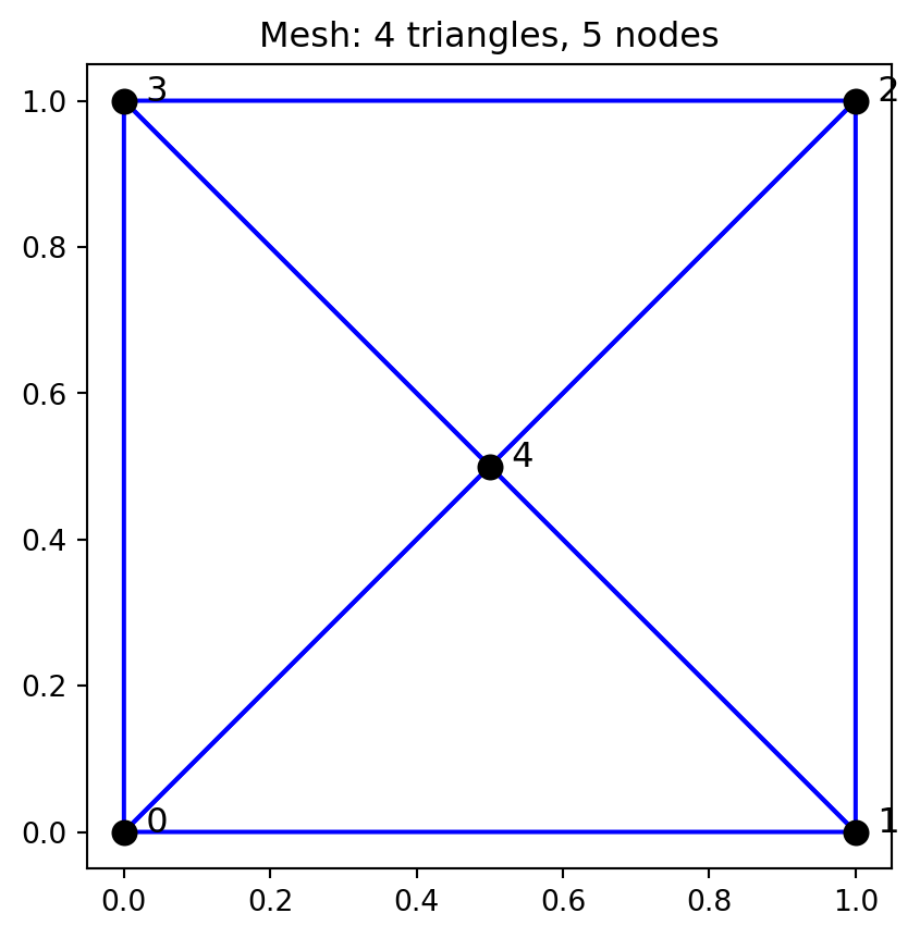

8.3 Step 3: Element-by-element assembly

The assembly loop scans through all elements, retrieves element matrices/vectors, and accumulates them into global arrays using the connectivity information.

ndofs = len(nodes)
K_global = np.zeros((ndofs, ndofs))
F_global = np.zeros(ndofs)
source_value = 1.0

for eid, conn in enumerate(elements):
    coords = nodes[list(conn)]
    x1v, y1v = coords[0]
    x2v, y2v = coords[1]
    x3v, y3v = coords[2]

    K_local = np.asarray(ke_fn(x1v, y1v, x2v, y2v, x3v, y3v), dtype=float)
    F_local = np.asarray(fe_fn(x1v, y1v, x2v, y2v, x3v, y3v, source_value), dtype=float).reshape(-1)

    print(f"Element {eid}, connectivity {conn}")
    print(f"  K_local diagonal: {np.diag(K_local)}")
    print(f"  F_local: {F_local}")

    assemble_dense_matrix(K_global, K_local, conn)
    assemble_dense_vector(F_global, F_local, conn)

print("\nAssembled K_global:")
print(np.round(K_global, 4))
print("\nAssembled F_global:")
print(np.round(F_global, 4))

Element 0, connectivity (0, 1, 4)
  K_local diagonal: [0.5 0.5 1. ]
  F_local: [0.08333333 0.08333333 0.08333333]
Element 1, connectivity (1, 2, 4)
  K_local diagonal: [0.5 0.5 1. ]
  F_local: [0.08333333 0.08333333 0.08333333]
Element 2, connectivity (2, 3, 4)
  K_local diagonal: [0.5 0.5 1. ]
  F_local: [0.08333333 0.08333333 0.08333333]
Element 3, connectivity (3, 0, 4)
  K_local diagonal: [0.5 0.5 1. ]
  F_local: [0.08333333 0.08333333 0.08333333]

Assembled K_global:
[[ 1.  0.  0.  0. -1.]
 [ 0.  1.  0.  0. -1.]
 [ 0.  0.  1.  0. -1.]
 [ 0.  0.  0.  1. -1.]
 [-1. -1. -1. -1.  4.]]

Assembled F_global:
[0.1667 0.1667 0.1667 0.1667 0.3333]

8.4 Step 4: Apply Dirichlet BCs and solve

Dirichlet boundary conditions are applied by reducing the system: we eliminate rows and columns corresponding to constrained DOFs and solve for the free DOFs, then expand the solution.

constrained = [0, 1, 2, 3]  # All boundary nodes
K_ff, F_f, free_dofs = apply_dirichlet_by_reduction(K_global, F_global, constrained)

print(f"Free DOFs: {free_dofs}")
print(f"K_ff = {K_ff}")
print(f"F_f = {F_f}")

u_free = np.linalg.solve(K_ff, F_f)
u = expand_reduced_solution(u_free, ndofs, free_dofs, constrained)

print(f"\nSolution vector u = {u}")
print(f"Center node value u[4] = {u[4]:.6f}")
print(f"Expected (analytical): 1/12 = {1/12:.6f}")
print(f"Match: {np.isclose(u[4], 1/12)}")

Free DOFs: [4]
K_ff = [[4.]]
F_f = [0.33333333]

Solution vector u = [0.         0.         0.         0.         0.08333333]
Center node value u[4] = 0.083333
Expected (analytical): 1/12 = 0.083333
Match: True

8.5 Step 5: Visualize the solution

We plot the FEM solution as a colored patch over the mesh, with annotations showing nodal values.

from matplotlib.tri import Triangulation

tri_conn = np.array(elements)
triang = Triangulation(nodes[:, 0], nodes[:, 1], tri_conn)

fig, ax = plt.subplots(figsize=(6, 5))
tpc = ax.tripcolor(triang, u, shading="flat", cmap="viridis")
ax.triplot(triang, "k-", linewidth=0.5)
for i, (x, y) in enumerate(nodes):
    ax.annotate(f"{i}: u={u[i]:.4f}", (x, y), fontsize=9,
                xytext=(5, 5), textcoords="offset points")
plt.colorbar(tpc, label="u")
ax.set_title("FEM Solution: Poisson on 4-Triangle Mesh")
ax.set_aspect("equal")
plt.show()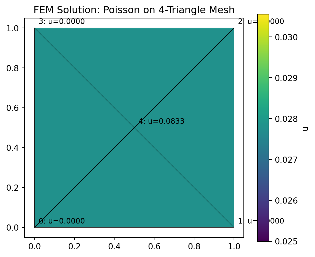

8.6 Exercise

Question: Move the center node from \((0.5, 0.5)\) to \((0.3, 0.7)\). How does the solution change? Is the center node value still \(1/12\)? Why or why not?

Hint: The center node is no longer at a symmetric position, so the Jacobians of the four elements are all different. This affects their stiffness matrices.

# Exercise: Move the center node from (0.5, 0.5) to (0.3, 0.7).
# How does the solution change? Is the center node value still 1/12?
# Why or why not?