7 L05 — Hyperelasticity
Strain Energy Functions, Isotropic Models, and Numerical Implementation
7.1 What is Hyperelasticity?
A material is hyperelastic (Green elastic) if there exists a strain energy function (SEF) \(W = \hat{W}(\mathbf{F})\) such that: \[ \mathbf{P} = \frac{\partial W}{\partial\mathbf{F}}, \qquad \mathbf{S} = 2\frac{\partial W}{\partial\mathbf{C}}. \]
This automatically satisfies the Clausius-Duhem inequality (no dissipation). Frame indifference restricts \(W\) to depend on \(\mathbf{F}\) only through \(\mathbf{C} = \mathbf{F}^T\mathbf{F}\).
7.2 Isotropy Restriction
For an isotropic hyperelastic material, \(W\) must depend only on the principal invariants of \(\mathbf{C}\) (or equivalently \(\mathbf{b}\)): \[ W = \hat{W}(I_1, I_2, I_3), \quad I_1 = \mathrm{tr}\,\mathbf{b}, \quad I_2 = \tfrac{1}{2}[(I_1)^2 - \mathrm{tr}\,\mathbf{b}^2], \quad I_3 = \det\mathbf{b} = J^2. \]
The Cauchy stress then follows: \[ \boldsymbol{\sigma} = \frac{2}{J}\left[ \left(\frac{\partial W}{\partial I_1} + I_1\frac{\partial W}{\partial I_2}\right)\mathbf{b} - \frac{\partial W}{\partial I_2}\mathbf{b}^2 + I_3\frac{\partial W}{\partial I_3}\mathbf{I} \right] \]
7.3 Compressible vs Incompressible Formulations
Incompressible: \(J = 1\) (constraint), introduce hydrostatic pressure \(p\) as Lagrange multiplier: \[ \boldsymbol{\sigma} = -p\mathbf{I} + 2\frac{\partial W}{\partial I_1}\mathbf{b} - 2\frac{\partial W}{\partial I_2}\mathbf{b}^{-1} \]
Compressible: use volumetric-isochoric split \(W = W_\text{vol}(J) + \bar{W}(\bar{I}_1, \bar{I}_2)\) where \(\bar{\mathbf{b}} = J^{-2/3}\mathbf{b}\) (unimodular part).
7.4 Neo-Hookean Model
The simplest physically motivated hyperelastic model: \[ W = \frac{\mu}{2}(I_1 - 3) - \mu\ln J + \frac{\lambda}{2}(\ln J)^2 \]
where \(\mu\) is the shear modulus and \(\lambda\) the first Lamé constant.
Cauchy stress: \[ \boldsymbol{\sigma} = \frac{\mu}{J}(\mathbf{b} - \mathbf{I}) + \frac{\lambda\ln J}{J}\mathbf{I} \]
Recovers linear elasticity at small strains.
7.5 Mooney-Rivlin Model
Two-parameter model for rubber-like materials: \[ W = C_1(I_1 - 3) + C_2(I_2 - 3) \] (incompressible form; add \(W_\text{vol}(J)\) for compressibility)
- \(C_1 = \mu/2\) in the Neo-Hookean limit (\(C_2 \to 0\))
- Better captures shear stiffening at moderate strains
- Experimental calibration: shear vs tension data
7.6 Ogden Model
General model written in terms of principal stretches \(\lambda_1, \lambda_2, \lambda_3\): \[ W = \sum_{p=1}^{N} \frac{\mu_p}{\alpha_p}\left(\lambda_1^{\alpha_p} + \lambda_2^{\alpha_p} + \lambda_3^{\alpha_p} - 3\right) \]
Conditions: \(\sum_p \mu_p\alpha_p > 0\) (positive initial shear modulus).
With \(N=3\) terms, fits vulcanized rubber data up to 700% extension.
7.7 Numerical Stress Computation
Algorithm for a given \(\mathbf{F}\):
def neo_hookean_stress(F, mu, lam):
    """Return Cauchy stress for compressible Neo-Hookean."""
    import numpy as np
    J = np.linalg.det(F)
    b = F @ F.T
    sigma = (mu / J) * (b - np.eye(3)) + (lam * np.log(J) / J) * np.eye(3)
    return sigma
7.8 Spatial Elasticity Tensor
Required by FEM for the consistent tangent. For the Neo-Hookean model:
\[ \mathbb{c} = \frac{\lambda}{J}\mathbf{I}\otimes\mathbf{I} + \frac{1}{J}\left(\mu - \lambda\ln J\right)(\mathbf{I}\overline{\otimes}\mathbf{I} + \mathbf{I}\underline{\otimes}\mathbf{I}) \]
where \((\mathbf{A}\overline{\otimes}\mathbf{B})_{ijkl} = A_{ik}B_{jl}\) and \((\mathbf{A}\underline{\otimes}\mathbf{B})_{ijkl} = A_{il}B_{jk}\).
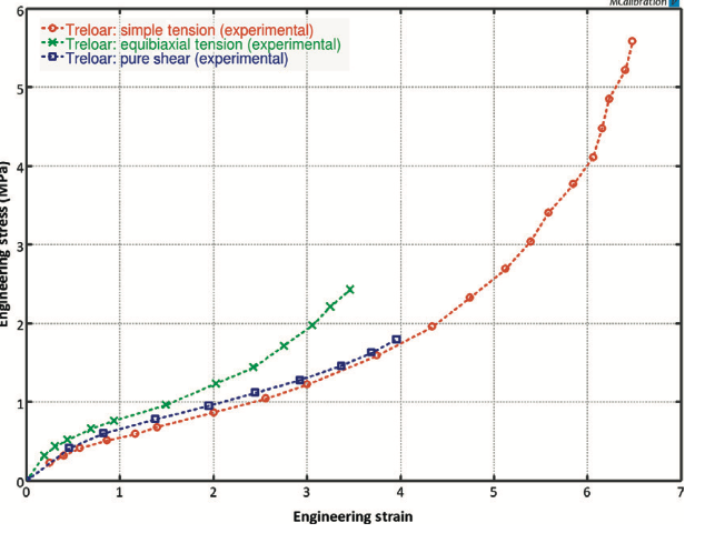
7.9 Treloar Data and Model Validation
The classic rubber dataset (Treloar 1944) tests models under combined loading:
- Uniaxial extension
- Equi-biaxial extension
- Pure shear
7.10 Rubber Elasticity: Molecular Origin
Definition: The ability of elastomers (polymeric materials) to undergo very large, reversible deformations under stress, returning quickly to their original shape upon unloading.
Key Characteristics: - Large strains (often several hundred percent) - Non-linear stress-strain behavior - Entropic in origin (unlike metallic elasticity which is enthalpic) - Low Young’s modulus, high Poisson’s ratio (\(\nu \approx 0.5\), nearly incompressible)
Temperature Dependence: Stiffness increases with temperature (consistent with entropic elasticity): \(G \propto T\).
7.11 Polymer Network Structure
Elastomers consist of long, flexible polymer chains linked together at specific crosslink points to form a 3D network.
Mechanism: - Unstressed State: Chains adopt random coil configurations (high entropy) - Stretched State: Chains are forced into more elongated, ordered configurations (low entropy). The network exerts a retractive force trying to return to the high-entropy state.
For elastomers, free energy is dominated by entropy: \[\Psi = \Psi_\text{internal} + \Psi_\text{entropy}, \quad \Psi_\text{entropy} = -\theta\eta\]
where \(\eta\) is entropy density. Stress arises from the tendency of chains to return to their random coil (highest entropy) state.
7.12 Incompressibility in Hyperelasticity
For rubber-like materials that are nearly incompressible, we use a volumetric-isochoric decomposition: \[W = W_\text{iso}(\bar{I}_1, \bar{I}_2) + W_\text{vol}(J)\]
where: - \(\bar{I}_1 = I_1 J^{-2/3}\), \(\bar{I}_2 = I_2 J^{-4/3}\) are the unimodular (volumetric-free) invariants - \(J = \det\mathbf{F} = \sqrt{I_3}\) is the volume ratio - \(W_\text{iso}\) captures shape change (deviatoric response) - \(W_\text{vol}\) captures volume change
For incompressible materials (\(J=1\)), we enforce this as a constraint, introducing hydrostatic pressure \(p\) as a Lagrange multiplier: \[\boldsymbol{\sigma} = -p\mathbf{I} + \boldsymbol{\sigma}_\text{dev}\]
where the deviatoric stress is derived from \(W_\text{iso}\).
7.13 Saint Venant-Kirchhoff Model
A simple linear model for the strain energy density: \[W = \frac{1}{2}\mathbf{E}:\mathbb{D}:\mathbf{E}\]
where \(\mathbb{D}\) is defined using Lamé parameters: \[\mathbb{D} = \lambda\mathbf{I}\otimes\mathbf{I} + 2\mu\mathbb{I}^4\]
with: \[\lambda = \frac{E\nu}{(1+\nu)(1-2\nu)}, \quad \mu = \frac{E}{2(1+\nu)}\]
Limitations: Valid only for small to moderate strains, despite using large-strain kinematics (Green-Lagrange strain).
Advantages: Can handle large rotations while remaining simple.
The second Piola-Kirchhoff stress is: \[\mathbf{S} = \frac{\partial W}{\partial\mathbf{E}} = 2\frac{\partial W}{\partial\mathbf{C}}\]
7.14 Relationship Between Stress Derivatives
Since \(\mathbf{E} = \frac{1}{2}(\mathbf{C} - \mathbf{I})\), we have: \[d\mathbf{E} = \frac{1}{2}d\mathbf{C}\]
The strain energy can be expressed in either form: \[d\Psi = \frac{\partial\Psi}{\partial\mathbf{E}} : d\mathbf{E} = \frac{\partial\Psi}{\partial\mathbf{C}} : d\mathbf{C}\]
Substituting \(d\mathbf{E} = \frac{1}{2}d\mathbf{C}\): \[\frac{\partial\Psi}{\partial\mathbf{E}} : \frac{1}{2}d\mathbf{C} = \frac{\partial\Psi}{\partial\mathbf{C}} : d\mathbf{C}\]
Since this holds for arbitrary \(d\mathbf{C}\): \[\mathbf{S} = \frac{\partial\Psi}{\partial\mathbf{E}} = 2\frac{\partial\Psi}{\partial\mathbf{C}}\]
7.15 Special Deformation Modes
For analyzing hyperelastic models, we often examine specialized deformations:
| Mode | Principal stretches | Definition |
|---|---|---|
| Uniaxial tension | \(\lambda_1 = \lambda\), \(\lambda_2 = \lambda_3 = \lambda^{-1/2}\) | Extension in one direction (incompressible) |
| Equibiaxial tension | \(\lambda_1 = \lambda_2 = \lambda\), \(\lambda_3 = \lambda^{-2}\) | Equal extension in two directions |
| Pure shear | \(\lambda_1 = \lambda\), \(\lambda_2 = \lambda^{-1}\), \(\lambda_3 = 1\) | Shear without volume change |
| Simple shear | \(\mathbf{F} = \mathbf{I} + \gamma\mathbf{e}_1\otimes\mathbf{e}_2\) | \(\gamma\) is shear strain |
These modes are used for model parameter fitting and validation against experimental data.
7.16 Gaussian Chain Statistics
A polymer chain can be modeled as an ideal random walk: - \(n\) rigid links of length \(l\) (total contour length \(L = nl\)) - End-to-end distance \(r\) with probability distribution - For Gaussian statistics (small extensions): \[P(r) = \left(\frac{3}{2\pi nl^2}\right)^{3/2} \exp\left(-\frac{3r^2}{2nl^2}\right)\]
The change in entropy for a network of chains is: \[\Delta\eta = -\frac{NK\theta}{2}(\lambda_1^2 + \lambda_2^2 + \lambda_3^2 - 3) = -W_G\]
where \(N\) is the number of chains, \(K\) is Boltzmann’s constant, and \(\theta\) is absolute temperature.
Limitations: Gaussian statistics assume freely jointed random coils, valid only for small to moderate stretches.
7.17 Non-Gaussian Chain Behavior
Real polymer chains have finite extensibility (maximum stretch \(\lambda_m\)). The force on a single stretched chain follows: \[f = \frac{NK\theta}{l}\mathbb{L}^{-1}\left(\frac{r}{nl}\right)\]
where \(\mathbb{L}^{-1}\) is the inverse Langevin function: \[\mathbb{L}(x) = 3x + \frac{9}{5}x^3 + \frac{297}{175}x^5 + \cdots\]
Key Property: \(\mathbb{L}^{-1}(x) \to \infty\) as \(x \to 1\), causing the force (and stress) to increase dramatically at high extensions.
This finite extensibility produces the characteristic “stiffening” (upturn) in the stress-strain curve at high strains, which Gaussian statistics cannot capture.
7.18 Arruda-Boyce (8-Chain) Model
Developed: Arruda and Boyce (1993) to capture finite extensibility using non-Gaussian statistics while remaining computationally simple.
Core Concept: Model the polymer network as a collection of identical unit cells, each containing 8 chains radiating from the center to the corners of a cube.
Deformation Assumption: - The cube vertices deform affinely with the macroscopic deformation - The 8 chains stretch according to the vertex displacements - This captures the average chain stretch in an isotropic network
The effective chain stretch is related to the first invariant: \[\lambda_\text{chain} = \sqrt{\frac{I_1}{3}}\]
Strain Energy Function: \[W_\text{AB} = NK\theta\sqrt{n} \left[ \lambda_\text{chain}\beta - \sqrt{n}\ln\left(\frac{\sinh\beta}{\beta}\right) \right]\]
where \(\beta = \mathbb{L}^{-1}(\lambda_\text{chain}/\sqrt{n})\) is related to the chain force.
Material Parameters: - \(N\) = number of segments per chain - \(K\) = Boltzmann constant - \(\theta\) = absolute temperature - Often simplified to two parameters: initial shear modulus and limiting stretch
7.19 Key Features of Arruda-Boyce
- Physical Basis: Directly incorporates finite chain extensibility
- Parameters: Only two interpretable material parameters
- Accuracy: Captures the characteristic ‘S-shape’ stress-strain curve including high-strain upturn
- Versatility: Performs well under various deformation modes (uniaxial, biaxial, shear) using the same parameters
- Implementation: Relatively straightforward to implement despite physical basis
7.20 Variational Formulation for Hyperelasticity
For a total Lagrangian (material) formulation, the total potential energy is: \[\Pi(\mathbf{u}) = \int_{\Omega_0} W(\mathbf{E}(\mathbf{u})) d\Omega_0 - \int_{\Omega_0} \mathbf{u}^T \mathbf{f}^b d\Omega_0 - \int_{\Gamma_{0,t}} \mathbf{u}^T \mathbf{t} d\Gamma_0\]
where \(\mathbf{f}^b\) is the body force and \(\mathbf{t}\) is the prescribed traction.
The first variation (Gâteaux derivative in direction \(\delta\mathbf{u}\)): \[\delta\Pi = \int_{\Omega_0} \mathbf{S} : \delta\mathbf{E} d\Omega_0 - \int_{\Omega_0} \delta\mathbf{u}^T \mathbf{f}^b d\Omega_0 - \int_{\Gamma_{0,t}} \delta\mathbf{u}^T \mathbf{t} d\Gamma_0\]
The Green-Lagrange strain variation (linear in \(\delta\mathbf{u}\), quadratic in \(\mathbf{u}\)): \[\delta\mathbf{E} = \operatorname{sym}((\nabla_0\mathbf{u})^T \nabla_0\delta\mathbf{u})\]
7.21 Linearization for Newton-Raphson
To solve the nonlinear system, we linearize around a current solution \(\mathbf{u}_i\) by taking the directional derivative in direction \(\Delta\mathbf{u}\):
\[\mathcal{L}[\delta\Pi] = \frac{d}{d\tau}\delta\Pi(\mathbf{u}_i + \tau\Delta\mathbf{u})\bigg|_{\tau=0}\]
The strain energy term linearizes as: \[\mathcal{L}\left[\int_{\Omega_0} \mathbf{S}:\delta\mathbf{E} d\Omega_0\right] = \int_{\Omega_0} [\Delta\mathbf{S}:\delta\mathbf{E} + \mathbf{S}:\Delta(\delta\mathbf{E})] d\Omega_0\]
where: - \(\Delta\mathbf{S} = \mathbb{D}:\Delta\mathbf{E}\) (material elasticity tensor \(\mathbb{D} = \frac{\partial\mathbf{S}}{\partial\mathbf{E}}\)) - \(\Delta\mathbf{E} = \operatorname{sym}((\nabla_0\mathbf{u})^T\nabla_0\Delta\mathbf{u})\) (increment of Green-Lagrange strain) - \(\Delta(\delta\mathbf{E}) = \operatorname{sym}((\nabla_0\Delta\mathbf{u})^T\nabla_0\delta\mathbf{u})\) (variation of strain increment)
The Newton-Raphson system at iteration \(k\) becomes: \[\int_{\Omega_0} [\mathbb{D}:\Delta\mathbf{E}:\delta\mathbf{E} + \mathbf{S}:\Delta(\delta\mathbf{E})] d\Omega_0 = -\mathcal{R}_k(\delta\mathbf{u})\]
where \(\mathcal{R}_k\) is the residual at iteration \(k\).
7.22 Material Elasticity Tensor
For the second Piola-Kirchhoff stress, the material elasticity tensor is: \[\mathbb{D}_{ijkl} = 4\frac{\partial^2 W}{\partial C_{ij}\partial C_{kl}}\]
This fourth-order tensor relates stress increments to strain increments: \[\Delta\mathbf{S} = \mathbb{D}:\Delta\mathbf{E}\]
For the Neo-Hookean model: \[W = \frac{\mu}{2}(I_1 - 3) - \mu\ln J + \frac{\lambda}{2}(\ln J)^2\]
The material elasticity tensor takes the form: \[\mathbb{D}_{ijkl} = \lambda\delta_{ij}\delta_{kl} + 2\mu\delta_{ik}\delta_{jl} + \mathcal{G}_{ijkl}\]
where \(\mathcal{G}\) includes additional terms from the volumetric part.