L05 — Hyperelasticity
Strain Energy Functions, Isotropic Models, and Numerical Implementation
📽 Slides: Open presentation
What is Hyperelasticity?
A material is hyperelastic (Green elastic) if there exists a strain energy function (SEF) \(W = \hat{W}(\mathbf{F})\) such that: \[ \mathbf{P} = \frac{\partial W}{\partial\mathbf{F}}, \qquad \mathbf{S} = 2\frac{\partial W}{\partial\mathbf{C}}. \]
This automatically satisfies the Clausius-Duhem inequality (no dissipation). Frame indifference restricts \(W\) to depend on \(\mathbf{F}\) only through \(\mathbf{C} = \mathbf{F}^T\mathbf{F}\).
Notation — reference vs current configuration. Following the course convention (see L03), uppercase symbols denote quantities defined on the reference (Lagrangian) configuration and lowercase symbols denote quantities defined on the current (Eulerian) configuration. In particular, the right Cauchy-Green tensor \(\mathbf{C} = \mathbf{F}^T\mathbf{F}\) is uppercase because it is a reference-frame quantity (pull-back of the spatial metric), while the left Cauchy-Green / Finger tensor \(\mathbf{b} = \mathbf{F}\mathbf{F}^T\) is lowercase because it is a current-frame quantity (push-forward of the reference metric). The two share the same principal invariants but live on different configurations.
Fourth-order elasticity tensors. The material (Lagrangian) tangent is \(\mathbb{D} = 2\,\partial\mathbf{S}/\partial\mathbf{C}\); its push-forward to the current configuration is \(\mathbb{c}\) (lowercase blackboard). Both are fourth-order. In L07–L09 plasticity chapters the 4th-order elasticity tensor is denoted \(\mathbb{C}^e\) (material); that is the small-strain specialisation of \(\mathbb{D}\).
Isotropy Restriction
For an isotropic hyperelastic material, \(W\) must depend only on the principal invariants of \(\mathbf{C}\) (or equivalently \(\mathbf{b}\)): \[ W = \hat{W}(I_1, I_2, I_3), \quad I_1 = \mathrm{tr}\,\mathbf{b}, \quad I_2 = \tfrac{1}{2}[(I_1)^2 - \mathrm{tr}\,\mathbf{b}^2], \quad I_3 = \det\mathbf{b} = J^2. \]
The Cauchy stress then follows: \[ \boldsymbol{\sigma} = \frac{2}{J}\left[ \left(\frac{\partial W}{\partial I_1} + I_1\frac{\partial W}{\partial I_2}\right)\mathbf{b} - \frac{\partial W}{\partial I_2}\mathbf{b}^2 + I_3\frac{\partial W}{\partial I_3}\mathbf{I} \right] \]
Compressible vs Incompressible Formulations
Incompressible: \(J = 1\) (constraint), introduce hydrostatic pressure \(p\) as Lagrange multiplier: \[ \boldsymbol{\sigma} = -p\mathbf{I} + 2\frac{\partial W}{\partial I_1}\mathbf{b} - 2\frac{\partial W}{\partial I_2}\mathbf{b}^{-1} \]
Compressible: use volumetric-isochoric split \(W = W_\text{vol}(J) + \bar{W}(\bar{I}_1, \bar{I}_2)\) where \(\bar{\mathbf{b}} = J^{-2/3}\mathbf{b}\) (unimodular part).
Neo-Hookean Model
The simplest physically motivated hyperelastic model: \[ W = \frac{\mu}{2}(I_1 - 3) - \mu\ln J + \frac{\lambda}{2}(\ln J)^2 \]
where \(\mu\) is the shear modulus and \(\lambda\) the first Lamé constant.
Cauchy stress: \[ \boldsymbol{\sigma} = \frac{\mu}{J}(\mathbf{b} - \mathbf{I}) + \frac{\lambda\ln J}{J}\mathbf{I} \]
Recovers linear elasticity at small strains.
Mooney-Rivlin Model
Two-parameter model for rubber-like materials: \[ W = C_1(I_1 - 3) + C_2(I_2 - 3) \] (incompressible form; add \(W_\text{vol}(J)\) for compressibility)
- \(C_1 = \mu/2\) in the Neo-Hookean limit (\(C_2 \to 0\))
- Better captures shear stiffening at moderate strains
- Experimental calibration: shear vs tension data
Ogden Model
General model written in terms of principal stretches \(\lambda_1, \lambda_2, \lambda_3\): \[ W = \sum_{p=1}^{N} \frac{\mu_p}{\alpha_p}\left(\lambda_1^{\alpha_p} + \lambda_2^{\alpha_p} + \lambda_3^{\alpha_p} - 3\right) \]
Conditions: \(\sum_p \mu_p\alpha_p > 0\) (positive initial shear modulus).
With \(N=3\) terms, fits vulcanized rubber data up to 700% extension.
Numerical Stress Computation
Algorithm for a given \(\mathbf{F}\):
Spatial Elasticity Tensor
Required by FEM for the consistent tangent. For the Neo-Hookean model:
\[ \mathbb{c} = \frac{\lambda}{J}\mathbf{I}\otimes\mathbf{I} + \frac{1}{J}\left(\mu - \lambda\ln J\right)(\mathbf{I}\overline{\otimes}\mathbf{I} + \mathbf{I}\underline{\otimes}\mathbf{I}) \]
where \((\mathbf{A}\overline{\otimes}\mathbf{B})_{ijkl} = A_{ik}B_{jl}\) and \((\mathbf{A}\underline{\otimes}\mathbf{B})_{ijkl} = A_{il}B_{jk}\).
Treloar Data and Model Validation
The classic rubber dataset (Treloar 1944) tests models under combined loading:
- Uniaxial extension
- Equi-biaxial extension
- Pure shear
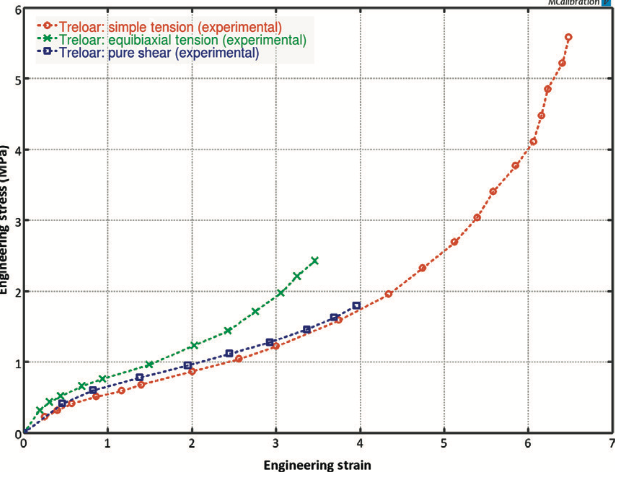
Treloar data fit comparison
Rubber Elasticity: Molecular Origin
Definition: The ability of elastomers (polymeric materials) to undergo very large, reversible deformations under stress, returning quickly to their original shape upon unloading.
Key Characteristics: - Large strains (often several hundred percent) - Non-linear stress-strain behavior - Entropic in origin (unlike metallic elasticity which is enthalpic) - Low Young’s modulus, high Poisson’s ratio (\(\nu \approx 0.5\), nearly incompressible)
Temperature Dependence: Stiffness increases with temperature (consistent with entropic elasticity): \(G \propto T\).
Polymer Network Structure
Elastomers consist of long, flexible polymer chains linked together at specific crosslink points to form a 3D network.
Mechanism: - Unstressed State: Chains adopt random coil configurations (high entropy) - Stretched State: Chains are forced into more elongated, ordered configurations (low entropy). The network exerts a retractive force trying to return to the high-entropy state.
For elastomers, free energy is dominated by entropy: \[\Psi = \Psi_\text{internal} + \Psi_\text{entropy}, \quad \Psi_\text{entropy} = -\theta\eta\]
where \(\eta\) is entropy density. Stress arises from the tendency of chains to return to their random coil (highest entropy) state.
Incompressibility in Hyperelasticity
For rubber-like materials that are nearly incompressible, we use a volumetric-isochoric decomposition: \[W = W_\text{iso}(\bar{I}_1, \bar{I}_2) + W_\text{vol}(J)\]
where: - \(\bar{I}_1 = I_1 J^{-2/3}\), \(\bar{I}_2 = I_2 J^{-4/3}\) are the unimodular (volumetric-free) invariants - \(J = \det\mathbf{F} = \sqrt{I_3}\) is the volume ratio - \(W_\text{iso}\) captures shape change (deviatoric response) - \(W_\text{vol}\) captures volume change
For incompressible materials (\(J=1\)), we enforce this as a constraint, introducing hydrostatic pressure \(p\) as a Lagrange multiplier: \[\boldsymbol{\sigma} = -p\mathbf{I} + \boldsymbol{\sigma}_\text{dev}\]
where the deviatoric stress is derived from \(W_\text{iso}\).
Saint Venant-Kirchhoff Model
A simple linear model for the strain energy density: \[W = \frac{1}{2}\mathbf{E}:\mathbb{D}:\mathbf{E}\]
where \(\mathbb{D}\) is defined using Lamé parameters: \[\mathbb{D} = \lambda\mathbf{I}\otimes\mathbf{I} + 2\mu\mathbb{I}^4\]
with: \[\lambda = \frac{E\nu}{(1+\nu)(1-2\nu)}, \quad \mu = \frac{E}{2(1+\nu)}\]
Limitations: Valid only for small to moderate strains, despite using large-strain kinematics (Green-Lagrange strain).
Advantages: Can handle large rotations while remaining simple.
The second Piola-Kirchhoff stress is: \[\mathbf{S} = \frac{\partial W}{\partial\mathbf{E}} = 2\frac{\partial W}{\partial\mathbf{C}}\]
Relationship Between Stress Derivatives
Since \(\mathbf{E} = \frac{1}{2}(\mathbf{C} - \mathbf{I})\), we have: \[d\mathbf{E} = \frac{1}{2}d\mathbf{C}\]
The strain energy can be expressed in either form: \[d\Psi = \frac{\partial\Psi}{\partial\mathbf{E}} : d\mathbf{E} = \frac{\partial\Psi}{\partial\mathbf{C}} : d\mathbf{C}\]
Substituting \(d\mathbf{E} = \frac{1}{2}d\mathbf{C}\): \[\frac{\partial\Psi}{\partial\mathbf{E}} : \frac{1}{2}d\mathbf{C} = \frac{\partial\Psi}{\partial\mathbf{C}} : d\mathbf{C}\]
Since this holds for arbitrary \(d\mathbf{C}\): \[\mathbf{S} = \frac{\partial\Psi}{\partial\mathbf{E}} = 2\frac{\partial\Psi}{\partial\mathbf{C}}\]
Special Deformation Modes
For analyzing hyperelastic models, we often examine specialized deformations:
| Mode | Principal stretches | Definition |
|---|---|---|
| Uniaxial tension | \(\lambda_1 = \lambda\), \(\lambda_2 = \lambda_3 = \lambda^{-1/2}\) | Extension in one direction (incompressible) |
| Equibiaxial tension | \(\lambda_1 = \lambda_2 = \lambda\), \(\lambda_3 = \lambda^{-2}\) | Equal extension in two directions |
| Pure shear | \(\lambda_1 = \lambda\), \(\lambda_2 = \lambda^{-1}\), \(\lambda_3 = 1\) | Shear without volume change |
| Simple shear | \(\mathbf{F} = \mathbf{I} + \gamma\mathbf{e}_1\otimes\mathbf{e}_2\) | \(\gamma\) is shear strain |
These modes are used for model parameter fitting and validation against experimental data.
Gaussian Chain Statistics
A polymer chain can be modeled as an ideal random walk: - \(n\) rigid links of length \(l\) (total contour length \(L = nl\)) - End-to-end distance \(r\) with probability distribution - For Gaussian statistics (small extensions): \[P(r) = \left(\frac{3}{2\pi nl^2}\right)^{3/2} \exp\left(-\frac{3r^2}{2nl^2}\right)\]
The change in entropy for a network of chains is: \[\Delta\eta = -\frac{NK\theta}{2}(\lambda_1^2 + \lambda_2^2 + \lambda_3^2 - 3) = -W_G\]
where \(N\) is the number of chains, \(K\) is Boltzmann’s constant, and \(\theta\) is absolute temperature.
Limitations: Gaussian statistics assume freely jointed random coils, valid only for small to moderate stretches.
Non-Gaussian Chain Behavior
Real polymer chains have finite extensibility (maximum stretch \(\lambda_m\)). The force on a single stretched chain follows: \[f = \frac{NK\theta}{l}\mathbb{L}^{-1}\left(\frac{r}{nl}\right)\]
where \(\mathbb{L}^{-1}\) is the inverse Langevin function: \[\mathbb{L}(x) = 3x + \frac{9}{5}x^3 + \frac{297}{175}x^5 + \cdots\]
Key Property: \(\mathbb{L}^{-1}(x) \to \infty\) as \(x \to 1\), causing the force (and stress) to increase dramatically at high extensions.
This finite extensibility produces the characteristic “stiffening” (upturn) in the stress-strain curve at high strains, which Gaussian statistics cannot capture.
Arruda-Boyce (8-Chain) Model
Developed: Arruda and Boyce (1993) to capture finite extensibility using non-Gaussian statistics while remaining computationally simple.
Core Concept: Model the polymer network as a collection of identical unit cells, each containing 8 chains radiating from the center to the corners of a cube.
Deformation Assumption: - The cube vertices deform affinely with the macroscopic deformation - The 8 chains stretch according to the vertex displacements - This captures the average chain stretch in an isotropic network
The effective chain stretch is related to the first invariant: \[\lambda_\text{chain} = \sqrt{\frac{I_1}{3}}\]
Strain Energy Function: \[W_\text{AB} = NK\theta\sqrt{n} \left[ \lambda_\text{chain}\beta - \sqrt{n}\ln\left(\frac{\sinh\beta}{\beta}\right) \right]\]
where \(\beta = \mathbb{L}^{-1}(\lambda_\text{chain}/\sqrt{n})\) is related to the chain force.
Material Parameters: - \(N\) = number of segments per chain - \(K\) = Boltzmann constant - \(\theta\) = absolute temperature - Often simplified to two parameters: initial shear modulus and limiting stretch
Key Features of Arruda-Boyce
- Physical Basis: Directly incorporates finite chain extensibility
- Parameters: Only two interpretable material parameters
- Accuracy: Captures the characteristic ‘S-shape’ stress-strain curve including high-strain upturn
- Versatility: Performs well under various deformation modes (uniaxial, biaxial, shear) using the same parameters
- Implementation: Relatively straightforward to implement despite physical basis
Variational Formulation for Hyperelasticity
For a total Lagrangian (material) formulation, the total potential energy is: \[\Pi(\mathbf{u}) = \int_{\Omega_0} W(\mathbf{E}(\mathbf{u})) d\Omega_0 - \int_{\Omega_0} \mathbf{u}^T \mathbf{f}^b d\Omega_0 - \int_{\Gamma_{0,t}} \mathbf{u}^T \mathbf{t} d\Gamma_0\]
where \(\mathbf{f}^b\) is the body force and \(\mathbf{t}\) is the prescribed traction.
The first variation (Gâteaux derivative in direction \(\delta\mathbf{u}\)): \[\delta\Pi = \int_{\Omega_0} \mathbf{S} : \delta\mathbf{E} d\Omega_0 - \int_{\Omega_0} \delta\mathbf{u}^T \mathbf{f}^b d\Omega_0 - \int_{\Gamma_{0,t}} \delta\mathbf{u}^T \mathbf{t} d\Gamma_0\]
The Green-Lagrange strain variation (linear in \(\delta\mathbf{u}\), quadratic in \(\mathbf{u}\)): \[\delta\mathbf{E} = \operatorname{sym}((\nabla_0\mathbf{u})^T \nabla_0\delta\mathbf{u})\]
Linearization for Newton-Raphson
To solve the nonlinear system, we linearize around a current solution \(\mathbf{u}_i\) by taking the directional derivative in direction \(\Delta\mathbf{u}\):
\[\mathcal{L}[\delta\Pi] = \frac{d}{d\tau}\delta\Pi(\mathbf{u}_i + \tau\Delta\mathbf{u})\bigg|_{\tau=0}\]
The strain energy term linearizes as: \[\mathcal{L}\left[\int_{\Omega_0} \mathbf{S}:\delta\mathbf{E} d\Omega_0\right] = \int_{\Omega_0} [\Delta\mathbf{S}:\delta\mathbf{E} + \mathbf{S}:\Delta(\delta\mathbf{E})] d\Omega_0\]
where: - \(\Delta\mathbf{S} = \mathbb{D}:\Delta\mathbf{E}\) (material elasticity tensor \(\mathbb{D} = \frac{\partial\mathbf{S}}{\partial\mathbf{E}}\)) - \(\Delta\mathbf{E} = \operatorname{sym}((\nabla_0\mathbf{u})^T\nabla_0\Delta\mathbf{u})\) (increment of Green-Lagrange strain) - \(\Delta(\delta\mathbf{E}) = \operatorname{sym}((\nabla_0\Delta\mathbf{u})^T\nabla_0\delta\mathbf{u})\) (variation of strain increment)
The Newton-Raphson system at iteration \(k\) becomes: \[\int_{\Omega_0} [\mathbb{D}:\Delta\mathbf{E}:\delta\mathbf{E} + \mathbf{S}:\Delta(\delta\mathbf{E})] d\Omega_0 = -\mathcal{R}_k(\delta\mathbf{u})\]
where \(\mathcal{R}_k\) is the residual at iteration \(k\).
Material Elasticity Tensor
For the second Piola-Kirchhoff stress, the material elasticity tensor is: \[\mathbb{D}_{ijkl} = 4\frac{\partial^2 W}{\partial C_{ij}\partial C_{kl}}\]
This fourth-order tensor relates stress increments to strain increments: \[\Delta\mathbf{S} = \mathbb{D}:\Delta\mathbf{E}\]
For the Neo-Hookean model: \[W = \frac{\mu}{2}(I_1 - 3) - \mu\ln J + \frac{\lambda}{2}(\ln J)^2\]
The material elasticity tensor takes the form: \[\mathbb{D}_{ijkl} = \lambda\delta_{ij}\delta_{kl} + 2\mu\delta_{ik}\delta_{jl} + \mathcal{G}_{ijkl}\]
where \(\mathcal{G}\) includes additional terms from the volumetric part.
Constitutive Models — Technion | Website