Code
try:
    import dolfinx
except ImportError:
    !wget "https://fem-on-colab.github.io/releases/fenicsx-install-release-real.sh" \
    -O "/tmp/fenicsx-install.sh" && bash "/tmp/fenicsx-install.sh"
import dolfinxWhat you’ve learned:
Derivvation of the weak form Simple linear problems Simple geometries Theoretical foundations Matrix formulations Direct solvers
Real engineering:
Complex 3D geometries Nonlinear materials Coupled physics Large-scale systems Complex boundary conditions Sophisticated solvers
FEniCSx bridges this gap!
Once you developed the weak form in its algebric form:
\[K \mathbf{u} = \mathbf{f}\]
FEniCSx handles:
Automatic mesh handling and partitioning
Assembly of \(K\) and \(\mathbf{f}\)
Efficient solvers (through external libraries like PETSc)
Post-processing
You focus on: Physics, boundary conditions, and engineering insight
High-level interface - Express problems in mathematical notation
Automatic (symbolic) differentiation
Access to advanced solvers and preconditioners
Parallel computing - Scales from laptop to supercomputer
Extensible - Custom materials, elements, and physics
In the following slides we will go through this workflow step by step.
The full code is available as a python file at the end of this presentation.
The problem on which we will demonstrate the workflow is a simple 2D beam bending problem.
The strong form of the problem is given as:
\[ - \nabla \cdot \sigma(u) = f \quad \text{in } \Omega \]
where \(\sigma\) is the stress tensor, \(u\) are the displacements \(\Omega\) the domain and \(f\) the body forces.
The constitutive relation, relating the displacements to the stress tensor is given as:
\[ \begin{aligned} \sigma(u) &= \lambda \text{tr}(\epsilon(u)) I + 2\mu \epsilon(u) \\ \epsilon(u) &= \nabla^s u \end{aligned} \]
with:
\[ \begin{aligned} \lambda &= \frac{E \nu}{(1+\nu)(1-2\nu)} \text{Lame's first parameter} \\ \mu &= \frac{E}{2(1+\nu)} \text{Lame's second parameter} \\ E &= \text{Young's modulus} \\ \nu &= \text{Poisson's ratio} \\ \nabla^s u &= \frac{1}{2}(\nabla u + \nabla^T u) \text{the symmetric gradient} \end{aligned} \]
The weak form of the problem is given as:
\[ \underbrace{\int_{\Omega} \sigma(u) : \epsilon(v) \, d\Omega}_{a(u,v)} = \underbrace{\int_{\Omega} f\cdot v \, d\Omega + \int_{\partial \Omega_T}T\cdot v \, d\partial \Omega_T}_{L(v)} \]
where \(v \in V\) is the test function (with \(V\) being the vector test function space), \(\partial \Omega_T\) is the part of the boundary on which tractions (\(T=\sigma \cdot n\)) are applied.
Rewriting the weak forms in terms of a linear and bilinear forms we can phrase the problem as:
Find \(u \in V\) such that:
\[ a(u,v) = L(v) \quad \forall v \in V \]
To run this example you will need to have FEniCSx installed on your system.
You can find the installation instructions on the FEniCSx website.
You can also use google’s Colab to run FEniCSx notebooks without having to install anything on your local machine.
Simply open a new notebook and run the following code to install FEniCSx:
try:
import dolfinx
except ImportError:
!wget "https://fem-on-colab.github.io/releases/fenicsx-install-release-real.sh" \
-O "/tmp/fenicsx-install.sh" && bash "/tmp/fenicsx-install.sh"
import dolfinxWe are using the python interface to FEniCSx - “dolfinx”
However, the same concepts apply to the C++ interface as well.
We will make use of the built-in meshe generator in FEniCSx to create a simple rectangular mesh for our beam.
We also import numpy and mpi4py for numerical operations and parallel computing, respectively.
from dolfinx import mesh
import ufl
import numpy as np
from mpi4py import MPI
# Define the geometry of the beam
Length = 20.0  # Length of the beam
Height = 1.0  # Height of the beam

Nx = 20  # Number of elements in the x-direction
Ny = 4  # Number of elements in the y-direction
#create the rectangular mesh
domain = mesh.create_rectangle(MPI.COMM_WORLD,
                            [np.array([0, 0]), np.array([Length, Height])],
                            [Nx, Ny],
                            cell_type=mesh.CellType.quadrilateral)
gdim = domain.geometry.dim # dimension Next, we define the function space for our problem.
We will use a vector function space with Lagrange elements of degree 1 (P1) for the displacements with gdim=2 since this is a 2D problem and we have \(u_x,u_y\).
from dolfinx import fem

# Define function space
Vdegree = 1  # Degree of the polynomial
V = fem.functionspace(domain, ("P", Vdegree, (gdim,)))
# V is a vector function space with gdim=2
# Vdegree=1 means linear elements (P1)

#Define the test and trial functions
u = ufl.TrialFunction(V)
v = ufl.TestFunction(V)We need to define the boundary conditions for our problem.
We will fix the left edge of the beam (x=0).
We do so by defining a function that identifies the left boundary and applying a Dirichlet boundary condition with zero displacement.
# Define Dirichlet boundary condition (fixed left edge)
def left_boundary(x):
    return np.isclose(x[0], 0)
#locate the dofs on the left boundary
fixed_side = fem.locate_dofs_geometrical(V, left_boundary)
# Define Dirichlet boundary condition
bc = [fem.dirichletbc(np.zeros(gdim), fixed_side, V)]from dolfinx import default_scalar_type
# Define body force (gravity)
rho = fem.Constant(domain, 2700.) # density of the material
g = fem.Constant(domain, 9.81) # gravitational acceleration
# Define body force vector
f = fem.Constant(domain, default_scalar_type((0, -rho * g)))In our problem definition we did not define any traction boundary conditions.
However, as an example, we show how to apply a spatially varying traction on the bottom surface of the beam.
def bottom_boundary(x):
return np.isclose(x[1], 0.0)
# Mark the boundaries with unique tags
fdim = gdim - 1 # The boundary dimension for 2D problems
bottom_facet = mesh.locate_entities_boundary(domain, fdim, bottom_boundary)
# Create a MeshTag: we tag the bottom boundary with a unique tag
bottom_tag = np.full_like(bottom_facet, 1)
facet_tag = mesh.meshtags(domain, fdim, bottom_facet, bottom_tag)
# Define a function for the tracitons
Traction_Function = fem.Function(V,name="Traction_Function")
# Define the traction function
tractions = lambda x: np.vstack((np.zeros_like(x[0],
dtype=default_scalar_type), -1.5 * x[0]))
# Assign the traction function to the Traction_Function
Traction_Function.interpolate(tractions)
# Define facet normal vector
n_vector = ufl.FacetNormal(domain)Now we can construct the weak form of the problem using the UFL (Unified Form Language) in FEniCSx which we prevously imported.
First, we need to define the integration measure for the boundary
# Define the integration measure for the boundary
ds = ufl.Measure("ds", domain=domain, subdomain_data=facet_tag)Now we are almost ready to define the bilinear form \(a(u,v)\) and the linear form \(L(v)\).
In the bilinear form, we have the integral of the stress tensor \(\sigma(u)\) multiplied by the symmetric gradient \(\epsilon(v)\)
So we will use the ufl module to define the stress tensor and the symmetric gradient.
Since we did not define the elastic properties of the material yet, we will do so now.
# Define material properties
E = fem.Constant(domain, 70e9) # Young's modulus in Pa
nu = fem.Constant(domain, 0.3) # Poisson's ratio
# Define Lame's parameters
lame = E * nu / ((1 + nu) * (1 - 2 * nu)) # Lame's first parameter
mu = E / (2 * (1 + nu)) # Lame's second parameter - shear modulus
def strain(v):
"""Define the strain tensor"""
return ufl.sym(ufl.grad(v)) # the symmetric gradient
def stress(u):
return lame * ufl.tr(strain(u))*ufl.Identity(gdim) + 2 * mu * strain(u)
# the stress tensorWe can now define the bilinear form \(a(u,v)\) and the linear form \(L(v)\).
# Define the bilinear form a(u,v)
a = ufl.inner(stress(u), strain(v)) * ufl.dx
# ufl.dx is the integration measure over the domain
# Define the linear form L(v)
# L = ufl.dot(f, v) * ufl.dx
# if you wish to apply the traction boundary condition you can
# add it to the linear form as follows:
L = ufl.dot(f, v) * ufl.dx + ufl.dot(Traction_Function,v) * ds(1)
# ds(1) is the integration measure over the bottom boundaryNote that we did not make use of the normal vector n_vector in the traction definition as we defined the traction as a vector operating in y direction and our boundary is straight in the x direction. for a curved boundary you would need to use the normal vector to define the traction in the correct direction.
FEniCSx contain has a “LinearProblem” class to handle the linear problem formulation.
from dolfinx.fem.petsc import LinearProblemWe can now create a LinearProblem object and solve the problem.
# Create the linear problem
problem = LinearProblem(a, L, bcs=bc,
petsc_options={"ksp_type": "preonly", "pc_type": "lu"})In the above code, we pass the bilinear form a, the linear form L, and the boundary conditions bc to the LinearProblem constructor.
We also specify some PETSc options for the solver, such as using a direct solver (ksp_type: preonly) and a LU factorization (pc_type: lu).
PETSc is a powerful library for solving linear systems and provides various solvers and preconditioners.
We can now solve the problem by calling the solve method of the LinearProblem object.
# Solve the linear problem
u_solution = problem.solve()The solve method returns the solution vector u_solution, which contains the displacements at each node of the mesh.
After solving the problem, we can visualize the results and extract useful information.
First, let’s visualize the displacements using the pyvista library, which is a powerful visualization library for Python.
import pyvista as pv
pv.OFF_SCREEN = True
from dolfinx import plot
pv.set_jupyter_backend('trame')
# Create a PyVista plotter
plotter = pv.Plotter()
# Create a PyVista mesh from the FEniCSx mesh
topology, cell_types, geometry = plot.vtk_mesh(V)
grid = pv.UnstructuredGrid(topology, cell_types, geometry)
#Since Pyvista expects a 3D vector field, we need to reshape the solution
u_2d = u_solution.x.array.reshape(geometry.shape[0], gdim)
u_3d = np.zeros((geometry.shape[0], 3))
u_3d[:, :gdim] = u_2d # Copy the x and y components
# Add the displacements ato the grid
grid["u"] = u_3d
# plot the undeformed mesh
undeformed = plotter.add_mesh(grid, style="wireframe", color="k")
# plot the deformed mesh
#create a warped mesh, and scale the displacements by a factor of your choice
factor = 10.
warped = grid.warp_by_vector("u",factor=factor)
#add the deformed mesh to the plotter
deformed = plotter.add_mesh(warped, show_edges=True)
plotter.show_axes()
#plot the two meshes.
if not pv.OFF_SCREEN:
plotter.show()
else:
disp_figure = plotter.screenshot("displacements.png")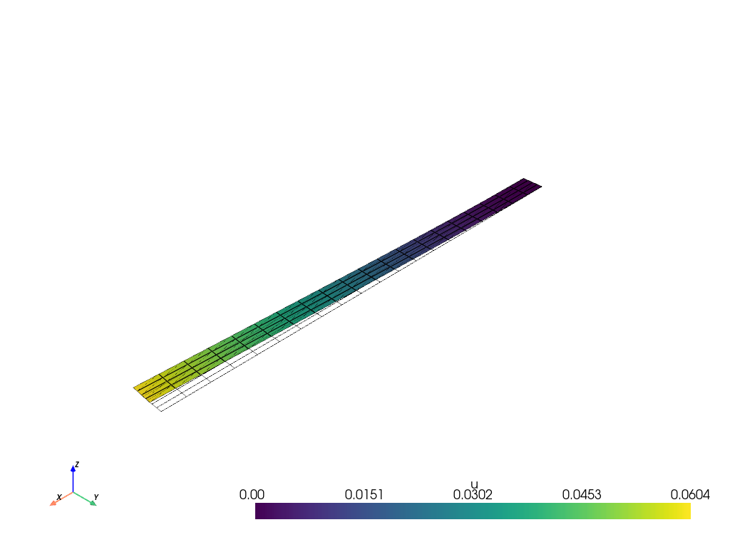
As you recall, the displacements are defined on the nodes of the mesh. To visualize the stress we need to project it onto the appropriate function space.
Let’s plot the Von Mises (or equivalent) stress.
# Compute the stress from the solution
stress_solution = stress(u_solution)
#transfer to deviatoric stress
deviatoric_stress = (stress_solution
- ufl.tr(stress_solution) / gdim * ufl.Identity(gdim))
# Compute the Von Mises stress
von_mises_stress = ufl.sqrt(3.0 / 2.0 *
ufl.inner(deviatoric_stress, deviatoric_stress))
# Create a FunctionSpace for the stress
stress_space = fem.functionspace(domain, ("DG", 0))
# Create an expression for the Von Mises stress
Mises_expression = fem.Expression(von_mises_stress,
stress_space.element.interpolation_points())
VM_stress = fem.Function(stress_space)
VM_stress.interpolate(Mises_expression)Now we can visualize the Von Mises stress using the pyvista library.
Note that now we assign values to the cells of the mesh (elements) instead of the nodes.
warped.cell_data["Von_Mises_Stress"] = VM_stress.x.array
warped.set_active_scalars("Von_Mises_Stress")
plotter = pv.Plotter()
plotter.add_mesh(warped)
plotter.show_axes()
if not pv.OFF_SCREEN:
plotter.show()
else:
VM_Stress_figure = plotter.screenshot(f"Von_Mises_Stress.png")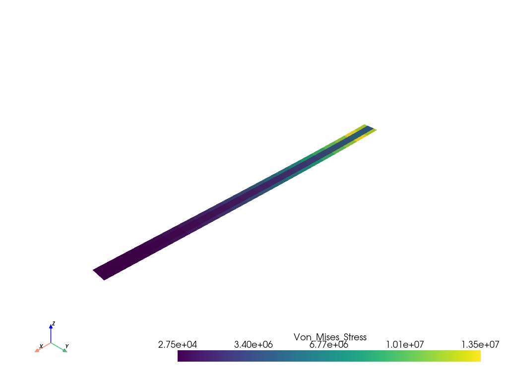
#%%
from dolfinx import mesh
import ufl
import numpy as np
from mpi4py import MPI
# Define the geometry of the beam
Length = 20.0 # Length of the beam
Height = 1.0 # Height of the beam
Nx = 20 # Number of elements in the x-direction
Ny = 4 # Number of elements in the y-direction
#create the rectangular mesh
domain = mesh.create_rectangle(MPI.COMM_WORLD,
[np.array([0, 0]), np.array([Length, Height])],
[Nx, Ny],
cell_type=mesh.CellType.quadrilateral)
gdim = domain.geometry.dim # dimension
#%%
from dolfinx import fem
# Define function space
Vdegree = 1 # Degree of the polynomial
V = fem.functionspace(domain, ("P", Vdegree, (gdim,)))
# V is a vector function space with gdim=2
# Vdegree=1 means linear elements (P1)
#Define the test and trial functions
u = ufl.TrialFunction(V)
v = ufl.TestFunction(V)
#%%
# Define Dirichlet boundary condition (fixed left edge)
def left_boundary(x):
return np.isclose(x[0], 0)
#locate the dofs on the left boundary
fixed_side = fem.locate_dofs_geometrical(V, left_boundary)
# Define Dirichlet boundary condition
bc = [fem.dirichletbc(np.zeros(gdim), fixed_side, V)]
#%%
from dolfinx import default_scalar_type
# Define body force (gravity)
rho = fem.Constant(domain, 2700.) # density of the material
g = fem.Constant(domain, 9.81) # gravitational acceleration
# Define body force vector
f = fem.Constant(domain, default_scalar_type((0, -rho * g)))
#%%
def bottom_boundary(x):
    return np.isclose(x[1], 0.0)
# Mark the boundaries with unique tags
fdim = gdim - 1  # The boundary dimension for 2D problems
bottom_facet = mesh.locate_entities_boundary(domain, fdim, bottom_boundary)
# Create a MeshTag: we tag the bottom boundary with a unique tag
bottom_tag = np.full_like(bottom_facet, 1)
facet_tag = mesh.meshtags(domain, fdim, bottom_facet, bottom_tag)
# Define a function for the tracitons
Traction_Function = fem.Function(V,name="Traction_Function")
# Define the traction function
tractions = lambda x: np.vstack((np.zeros_like(x[0],
                        dtype=default_scalar_type), -1.5 * x[0]))
# Assign the traction function to the Traction_Function
Traction_Function.interpolate(tractions)
# Define facet normal vector
n_vector = ufl.FacetNormal(domain)
#%%
ds = ufl.Measure("ds", domain=domain, subdomain_data=facet_tag)
# Define material properties
E = fem.Constant(domain, 70e9)  # Young's modulus in Pa
nu = fem.Constant(domain, 0.3)  # Poisson's ratio
# Define Lame's parameters
lame = E * nu / ((1 + nu) * (1 - 2 * nu))  # Lame's first parameter
mu = E / (2 * (1 + nu))  # Lame's second parameter - shear modulus

def strain(v):
    """Define the strain tensor"""
    return ufl.sym(ufl.grad(v)) # the symmetric gradient

def stress(u):
     return lame * ufl.tr(strain(u))*ufl.Identity(gdim) + 2 * mu * strain(u)
     # the stress tensor
#%%
# Define the bilinear form a(u,v)
a = ufl.inner(stress(u), strain(v)) * ufl.dx
# ufl.dx is the integration measure over the domain

# Define the linear form L(v)
# L = ufl.dot(f, v) * ufl.dx

# if you wish to apply the traction boundary condition you can
# add it to the linear form as follows:
L = ufl.dot(f, v) * ufl.dx  + ufl.dot(Traction_Function,v) * ds(1)
# ds(1) is the integration measure over the bottom boundary
#%%
from dolfinx.fem.petsc import LinearProblem
problem = LinearProblem(a, L, bcs=bc,
petsc_options={"ksp_type": "preonly", "pc_type": "lu"})
u_solution = problem.solve()
#%%
import pyvista as pv
from dolfinx import plot
pv.set_jupyter_backend('trame')
# Create a PyVista plotter
plotter = pv.Plotter()
# Create a PyVista mesh from the FEniCSx mesh
topology, cell_types, geometry = plot.vtk_mesh(V)
grid = pv.UnstructuredGrid(topology, cell_types, geometry)
#Since Pyvista expects a 3D vector field, we need to reshape the solution
u_2d = u_solution.x.array.reshape(geometry.shape[0], gdim)
u_3d = np.zeros((geometry.shape[0], 3))
u_3d[:, :gdim] = u_2d # Copy the x and y components
# Add the displacements ato the grid
grid["u"] = u_3d
# plot the undeformed mesh
undeformed = plotter.add_mesh(grid, style="wireframe", color="k")
# plot the deformed mesh
#create a warped mesh, and scale the displacements by a factor of your choice
factor = 10.
warped = grid.warp_by_vector("u",factor=factor)
#add the deformed mesh to the plotter
deformed = plotter.add_mesh(warped, show_edges=True)
plotter.show_axes()
#plot the two meshes.
if not pv.OFF_SCREEN:
plotter.show()
else:
disp_figure = plotter.screenshot("displacements.png")
#%%
# Compute the stress from the solution
stress_solution = stress(u_solution)
#transfer to deviatoric stress
deviatoric_stress = (stress_solution
                    - ufl.tr(stress_solution) / gdim * ufl.Identity(gdim))
# Compute the Von Mises stress
von_mises_stress = ufl.sqrt(3.0 / 2.0 *
                        ufl.inner(deviatoric_stress, deviatoric_stress))
# Create a FunctionSpace for the stress
stress_space = fem.functionspace(domain, ("DG", 0))
# Create an expression for the Von Mises stress
Mises_expression = fem.Expression(von_mises_stress,
                                stress_space.element.interpolation_points())
VM_stress = fem.Function(stress_space)
VM_stress.interpolate(Mises_expression)
#%%
warped.cell_data["Von_Mises_Stress"] = VM_stress.x.array
warped.set_active_scalars("Von_Mises_Stress")
plotter = pv.Plotter()
plotter.add_mesh(warped)
plotter.show_axes()
if not pv.OFF_SCREEN:
    plotter.show()
else:
    VM_Stress_figure = plotter.screenshot(f"Von_Mises_Stress.png")
# %%