L09 — Damage Mechanics

Continuum Damage, Fracture, and Coupled Problems

📽 Slides: Open presentation

This chapter covers two coupled mechanics frameworks. (1) Continuum Damage Mechanics (CDM) — introduces a scalar damage variable \(D \in [0,1]\) that degrades elastic stiffness. (2) Pressure-dependent plasticity — Drucker-Prager and Mohr-Coulomb yield criteria that incorporate hydrostatic stress via \(I_1\) or \(p\). The two can be combined in coupled damage-plasticity models.

Regime. Unless stated otherwise, this chapter (and L08, L09) assumes the small-strain regime: \(\boldsymbol{\varepsilon} = \tfrac{1}{2}(\nabla\mathbf{u} + \nabla\mathbf{u}^T)\), with additive decomposition \(\boldsymbol{\varepsilon} = \boldsymbol{\varepsilon}^e + \boldsymbol{\varepsilon}^p\). Finite-strain plasticity uses a multiplicative split \(\mathbf{F} = \mathbf{F}^e\mathbf{F}^p\) (outside scope).

Motivation: Degradation of Stiffness

Unlike plasticity (permanent strain), damage describes the progressive degradation of material stiffness due to microcrack growth and void coalescence.

Observable signatures:

• Reduction of the elastic modulus
• Stress softening (load-bearing capacity decreases with deformation)
• Final fracture / failure

Continuum Damage Mechanics (CDM) describes this via internal damage variables without resolving individual cracks.

Isotropic Damage Model

A scalar damage variable \(D \in [0, 1]\):

• \(D = 0\): virgin (undamaged) material
• \(D = 1\): fully damaged (no load-carrying capacity)

Effective stress concept (Lemaitre): \[ \tilde{\boldsymbol{\sigma}} = \frac{\boldsymbol{\sigma}}{1-D} \]

Constitutive law with damage: \[ \boldsymbol{\sigma} = (1-D)\,\mathbb{C}^e:\boldsymbol{\varepsilon} \]

Strain Equivalence Principle

Strain equivalence (Lemaitre): the strain in the damaged material under nominal stress \(\boldsymbol{\sigma}\) equals the strain in the undamaged material under effective stress \(\tilde{\boldsymbol{\sigma}}\).

This allows re-use of undamaged material models by simply replacing \(\boldsymbol{\sigma} \to \tilde{\boldsymbol{\sigma}}\).

Energy equivalence (Cordebois & Sidoroff): alternative that gives different predictions for shear.

Damage Evolution Law

Thermodynamic driving force (energy release rate \(Y\)): \[ Y = -\frac{\partial\Psi}{\partial D} = \frac{1}{2}\boldsymbol{\varepsilon}:\mathbb{C}^e:\boldsymbol{\varepsilon} \]

Damage criterion and evolution: \[ g(Y, D) = Y - r(D) \leq 0, \qquad \dot{D} = \dot{\mu}\frac{\partial g}{\partial Y}, \]

where \(r(D)\) is the damage threshold function (analogous to yield stress hardening).

Coupling Damage with Plasticity

Combined elasto-plastic-damage model free energy: \[ \Psi = (1-D)\hat{\Psi}^e(\boldsymbol{\varepsilon}^e) + \Psi^p(\bar{\varepsilon}^p) \]

The stress: \[ \boldsymbol{\sigma} = (1-D)\mathbb{C}^e:\boldsymbol{\varepsilon}^e \]

Both yield surface and damage criterion must be checked at each step. Order of priority depends on the coupling model chosen.

Softening and Regularization

Softening (negative tangent modulus) triggers:

• Loss of ellipticity of governing equations
• Mesh-dependent FEM solutions (localization into a band of one element width)

Regularization methods:

• Nonlocal damage: replace \(Y\) by a weighted spatial average \(\bar{Y}\)
• Gradient damage: add \(-c\,\Delta D\) to the damage driving force
• Phase-field fracture: variational approach with intrinsic length scale

Phase-Field Approach to Fracture

Introduce a smooth phase-field \(\phi \in [0,1]\) interpolating between intact (\(\phi=0\)) and fractured (\(\phi=1\)):

\[ \mathcal{E}(\mathbf{u}, \phi) = \int_\Omega \left[ g(\phi)\Psi^e_+(\boldsymbol{\varepsilon}) + \Psi^e_-(\boldsymbol{\varepsilon}) + \frac{G_c}{2}\left(\frac{\phi^2}{l_0} + l_0|\nabla\phi|^2\right) \right]dV \]

where \(g(\phi) = (1-\phi)^2\) is the degradation function and \(l_0\) the regularization length.

Advantages: no explicit crack tracking, natural branching/merging.

Thermo-Mechanical Coupling

Temperature \(\theta\) affects yield stress and elastic moduli: \[ \sigma_y = \sigma_y(\bar{\varepsilon}^p, \theta), \qquad \boldsymbol{\varepsilon}^\text{th} = \alpha(\theta - \theta_\text{ref})\mathbf{I}. \]

Energy equation with heat generated by plastic dissipation (Taylor-Quinney coefficient \(\beta \approx 0.9\)): \[ \rho c_p\dot{\theta} = \beta\,\boldsymbol{\sigma}:\dot{\boldsymbol{\varepsilon}}^p + \nabla\cdot(k\nabla\theta) \]

Strong coupling requires staggered or monolithic FEM solvers.

Pressure-Dependent Yield Criteria (Recap)

Materials like soils, rocks, and concrete exhibit plastic behavior that depends strongly on hydrostatic pressure, unlike metals (which follow von Mises, pressure-independent).

Why Pressure Dependence Matters: - Frictional effects: higher normal stress increases shear strength - Dilatational effects: volume changes coupled to plastic flow - Confinement: material becomes stronger under compression

All pressure-dependent models consist of: 1. Additive strain decomposition: \(\boldsymbol{\varepsilon} = \boldsymbol{\varepsilon}^e + \boldsymbol{\varepsilon}^p\) 2. Hypoelastic law: \(\dot{\boldsymbol{\sigma}} = \mathbb{C}^e : \dot{\boldsymbol{\varepsilon}}^e\) 3. Yield function: \(f(\boldsymbol{\sigma}, q) \leq 0\) (depends on hydrostatic pressure \(p\)) 4. Flow rule: \(\dot{\boldsymbol{\varepsilon}}^p = \dot{\gamma} \frac{\partial g(\boldsymbol{\sigma}, q)}{\partial\boldsymbol{\sigma}}\) (often non-associative: \(g \neq f\)) 5. Hardening law: \(\dot{q} = \dot{\gamma} h(\boldsymbol{\sigma}, q)\) (e.g., cohesion increases with plastic strain) 6. Kuhn-Tucker conditions: \(\dot{\gamma} \geq 0\), \(f \leq 0\), \(\dot{\gamma}f = 0\)

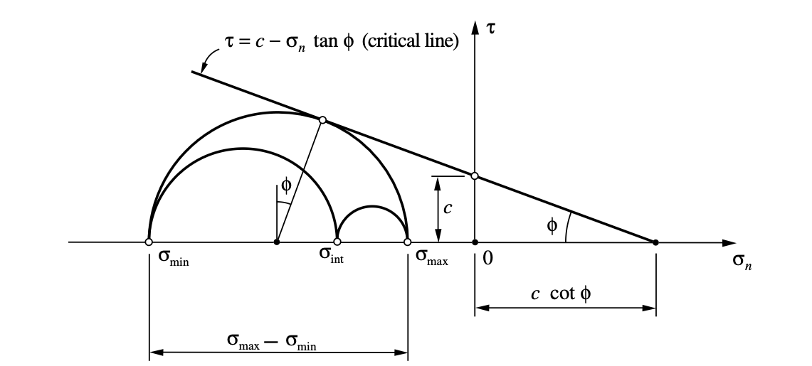
Mohr-Coulomb Criterion

The Mohr-Coulomb criterion is the classical model for frictional materials (soils, rocks, concrete).

Physical Interpretation: Yielding occurs when shear stress on any plane reaches: \[\tau = c - \sigma_n\tan\phi\]

where: - \(\tau\) = shear stress on the failing plane - \(\sigma_n\) = normal stress on the failing plane - \(c\) = cohesion (material strength when \(\sigma_n = 0\)) - \(\phi\) = internal friction angle

This gives a linear failure envelope in \((\sigma_n, \tau)\) space.

Yield Function in Terms of Principal Stresses:

For principal stresses \(\sigma_1 \geq \sigma_2 \geq \sigma_3\): \[\Phi(\boldsymbol{\sigma}, c) = (\sigma_1 - \sigma_3) + (\sigma_1 + \sigma_3)\sin\phi - 2c\cos\phi = 0\]

Using invariants (with \(p\) = mean pressure, \(\theta\) = Lode angle, \(J_2, J_3\) = stress invariants): \[\Phi = \left(\cos\theta - \frac{\sin\theta\sin\phi}{\sqrt{3}}\right)\sqrt{J_2} + p\sin\phi - c\cos\phi = 0\]

Key Properties: - Non-smooth yield surface: hexagonal pyramid in principal stress space - Apex at \(p = c\cot\phi\) (tensile limit) - Generally non-associative flow rule (dilation angle \(\psi \neq \phi\)) - Hardening: cohesion becomes a function of accumulated plastic strain: \(c = c(\bar{\varepsilon}^p)\)

Mohr-Coulomb surface

Tresca Criterion

The Tresca yield criterion (pressure-insensitive version of M-C) states that plasticity begins when the maximum shear stress reaches a critical value:

\[\tau_{\max} = \frac{1}{2}(\sigma_{\max} - \sigma_{\min})\]

Yield Function: \[\Phi(\boldsymbol{\sigma}) = (\sigma_1 - \sigma_3) - \sigma_y(\bar{\varepsilon}^p) = 0\]

where \(\sigma_y(\bar{\varepsilon}^p)\) is the uniaxial yield stress (function of hardening variable \(\bar{\varepsilon}^p\)).

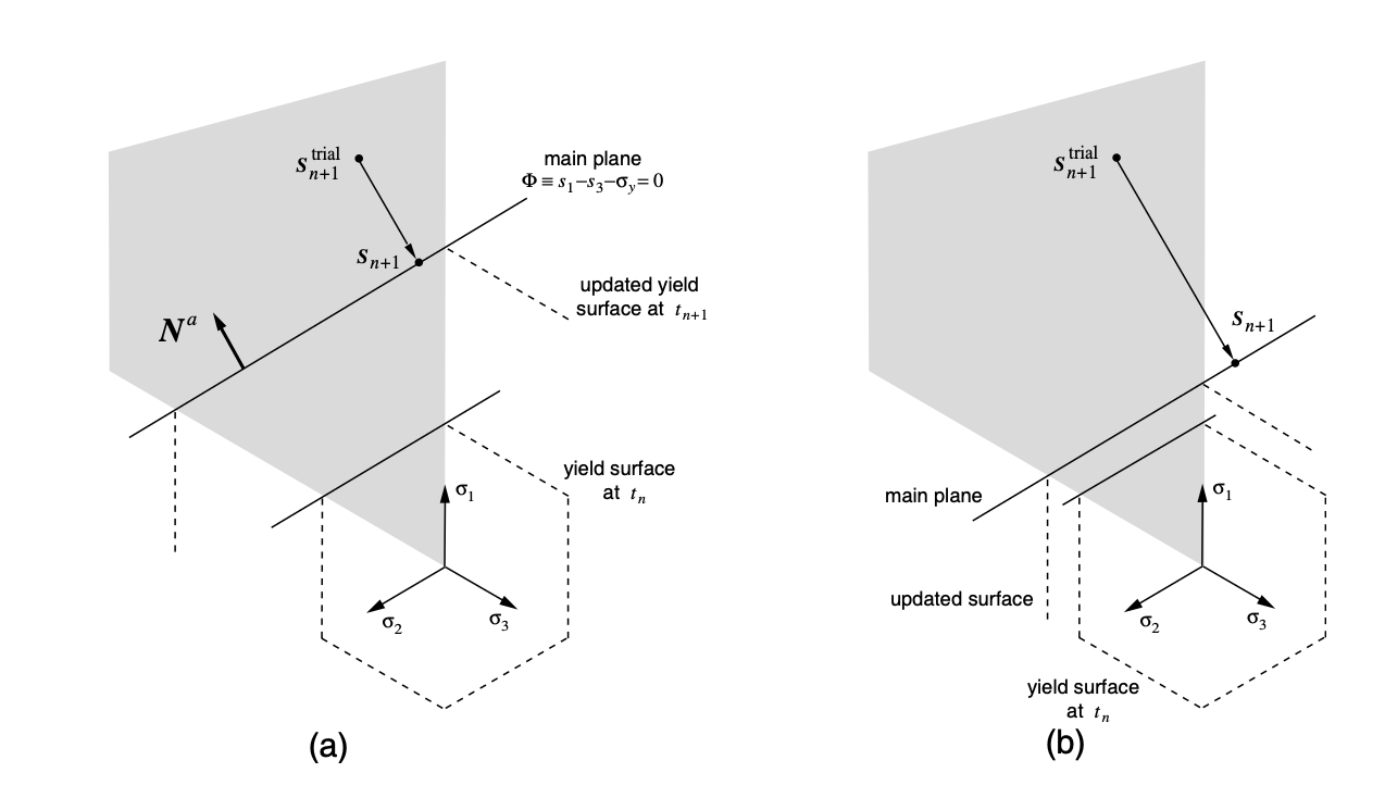
Yield Surface: A hexagonal prism in principal stress space (axis = hydrostatic line).

Multisurface Representation: Six yield surfaces based on principal stress pairs: \[\Phi_1 = \sigma_1 - \sigma_3 - \sigma_y, \quad \Phi_2 = \sigma_2 - \sigma_3 - \sigma_y, \quad \Phi_3 = \sigma_1 - \sigma_2 - \sigma_y, \ldots\]

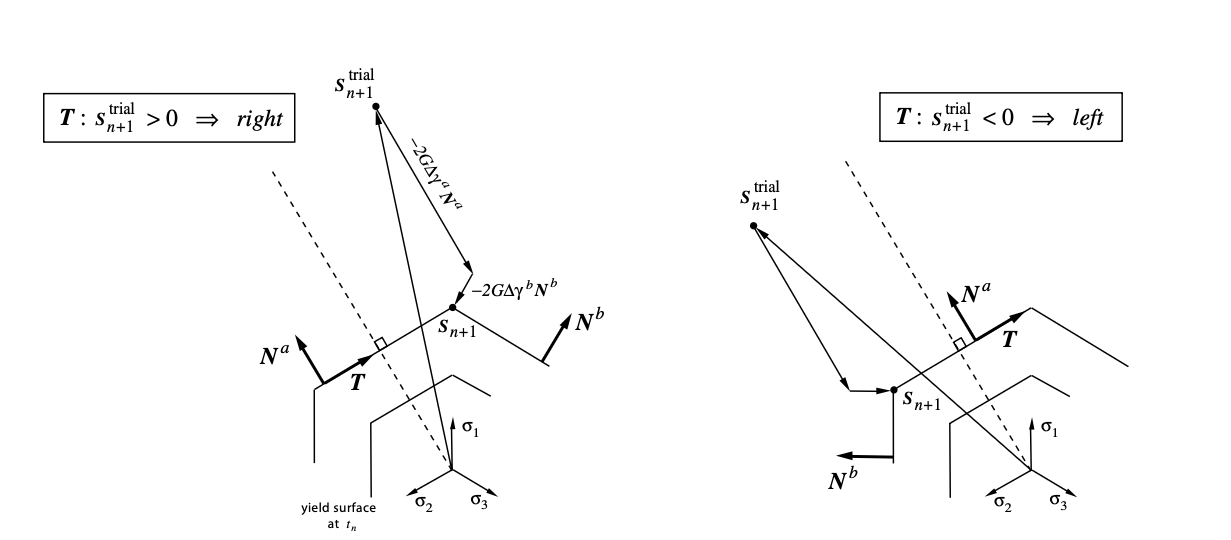
Only one or two surfaces are active at a given stress state; the algorithm must identify the active subset.

Return Mapping Procedure:

For a given principal stress ordering (\(\sigma_1 \geq \sigma_2 \geq \sigma_3\)), three cases arise:

1. Main plane flow (\(\Phi_1\) only): one multiplier \(\Delta\gamma\)
   • Updates: \(s_1 = s_{trial,1} - 2G\Delta\gamma\), \(s_3 = s_{trial,3} + 2G\Delta\gamma\), \(s_2\) unchanged
   • Consistency: \(s_{trial,1} - s_{trial,3} - 4G\Delta\gamma - \sigma_y(\bar{\varepsilon}_{p,n} + \Delta\gamma) = 0\)
2. Corner flow (two surfaces active, e.g., \(\Phi_1\) and \(\Phi_6\)): two multipliers \(\Delta\gamma_a, \Delta\gamma_b\)
   • More complex stress updates and consistency conditions (system of 2 equations)
3. Another corner (\(\Phi_1\) and \(\Phi_2\)): similar to case 2 but different geometry

The algorithm must determine which case applies and solve accordingly (often with iteration).

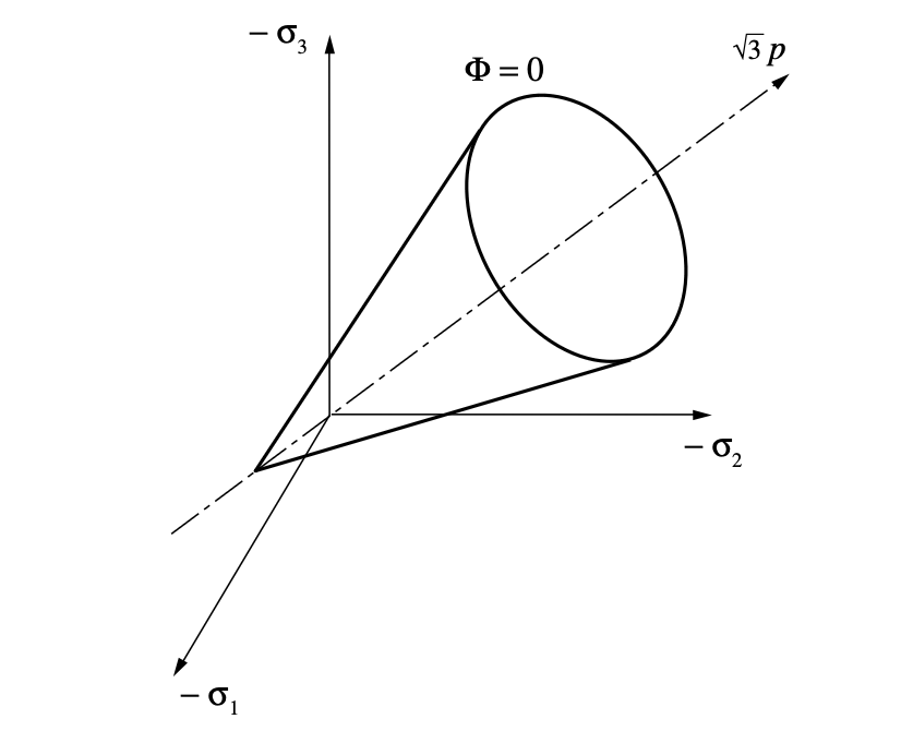
Drucker-Prager Criterion

The Drucker-Prager (DP) criterion is a smooth approximation to Mohr-Coulomb, incorporating pressure into a von Mises-like framework.

Yield Function: \[f_\text{DP}(\boldsymbol{\sigma}, c) = \sqrt{J_2(\mathbf{s}(\boldsymbol{\sigma}))} + \eta\, p(\boldsymbol{\sigma}) - \xi\, c = 0\]

where: - \(\sqrt{J_2}\) = equivalent deviatoric stress (like von Mises) - \(p\) = hydrostatic pressure - \(\eta, \xi\) = material parameters chosen to fit Mohr-Coulomb - \(c = c(\bar{\varepsilon}^p)\) = cohesion (hardening variable)

Yield Surface: A circular cone in principal stress space (smooth, isotropic about hydrostatic axis).

Advantages over M-C: - Smooth (no corners) → simpler numerical implementation - No need for multisurface logic - Single elastic region identification

Flow Rule (Non-Associative):

The flow potential is: \[\Psi(\boldsymbol{\sigma}, c) = \sqrt{J_2(\mathbf{s})} + \bar{\eta} p\]

Flow vector: \[\mathbf{N} = \frac{\partial\Psi}{\partial\boldsymbol{\sigma}} = \frac{\mathbf{s}}{2\sqrt{J_2}} + \frac{\bar{\eta}}{3}\mathbf{I}\]

where the second term represents volumetric (dilatational) flow. The dilatancy parameter \(\bar{\eta}\) can differ from \(\eta\) in the yield function.

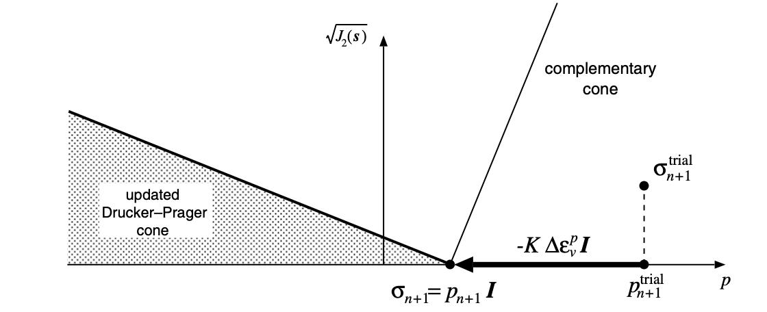
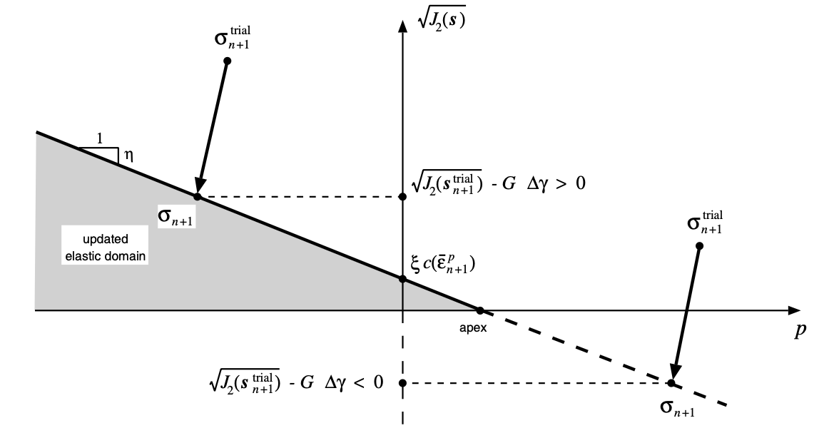
Return Mapping Algorithm:

Two cases exist due to cone geometry:

1. Return to smooth cone portion:
   • Update deviatoric stress: \(\mathbf{s}_{n+1} = \left(1 - \frac{G\Delta\gamma}{\sqrt{J_2(s_{trial})}}\right) \mathbf{s}_{trial}\)
   • Update mean pressure: \(p_{n+1} = p_{trial} - K\bar{\eta}\Delta\gamma\)
   • Consistency condition gives scalar equation for \(\Delta\gamma\)
2. Return to apex (when stress tries to enter the “forbidden” region):
   • Deviatoric stress collapses: \(\mathbf{s}_{n+1} = 0\)
   • Mean pressure determined from apex condition: \(p = \frac{\xi}{\eta}c\)
   • Different scalar equation for volumetric plastic strain increment

The algorithm first attempts the smooth cone; if invalid, it applies the apex return.

Consistent Tangent Moduli

For Newton-Raphson convergence in FEM, we need the algorithmic (consistent) tangent stiffness \(\mathbb{C}_{\text{ep}}\).

For Drucker-Prager (Smooth Cone Return): \[\mathbb{C}_{\text{ep}} = 2G\left(1 - \frac{\Delta\gamma}{\sqrt{2}\|\varepsilon^e_{trial,\text{dev}}\|}\right)\mathbb{I}_{\text{dev}} + 2G\left(\frac{\Delta\gamma}{\sqrt{2}\|\varepsilon^e_{trial,\text{dev}}\|} - GA\right)\mathbf{D}\otimes\mathbf{D}\] \[\quad - \sqrt{2}GAK(\eta\mathbf{D}\otimes\mathbf{I} + \bar{\eta}\mathbf{I}\otimes\mathbf{D}) + K(1 - K\eta\bar{\eta}A)\mathbf{I}\otimes\mathbf{I}\]

where \(A = \frac{1}{G + K\eta\bar{\eta} + \xi^2 H_\text{iso}}\) and \(H_\text{iso}\) is the hardening slope.

For Drucker-Prager (Apex Return): \[\mathbb{C}_{\text{ep}} = K\left(1 - \frac{K}{K + \alpha^2 H_\text{iso}}\right)\mathbf{I}\otimes\mathbf{I}\]

where \(\alpha = \xi/\bar{\eta}\).

The algorithm uses the tangent consistent with the return mapping (smooth or apex) that was active in the previous iteration.

Mohr-Coulomb and Drucker-Prager: Key Relationships

Material parameters can be related via:

Parameter	Expression
\(\eta\) (DP yield)	\(\sin\phi / \sqrt{9 + 3\sin^2\phi}\)
\(\xi\) (DP yield)	\(3c\cos\phi / \sqrt{9 + 3\sin^2\phi}\)
\(\bar{\eta}\) (DP flow)	Often chosen as \(\sin\psi\) (dilatancy angle)

These relationships allow fitting Drucker-Prager parameters to match Mohr-Coulomb behavior while maintaining smoothness for numerical robustness.