L03 — Continuum Kinematics
Deformation, Strain Measures, and Stress Tensors
Sign convention. The Cauchy stress \(\boldsymbol{\sigma}\) is positive in tension and negative in compression throughout this course. The hydrostatic pressure is \(p = -\tfrac{1}{3}\operatorname{tr}\boldsymbol{\sigma}\) (so positive \(p\) means compression).
Notation from this chapter onwards. Direct tensor notation (e.g. \(\mathbf{F}\), \(\boldsymbol{\sigma}\), \(\mathbb{C}^e\)) is used predominantly; index notation (\(F_{iJ}\), \(\sigma_{ij}\), \(C^e_{ijkl}\)) is shown where clarity requires it. Bold Latin uppercase denotes reference-configuration second-order tensors (\(\mathbf{F}\), \(\mathbf{C}\), \(\mathbf{E}\)); bold Latin lowercase denotes current-configuration second-order tensors (\(\mathbf{b}\), \(\mathbf{e}\)); blackboard bold (\(\mathbb{C}\), \(\mathbb{P}\)) denotes fourth-order tensors. See L02 for the index-notation toolkit.
The Deformation Gradient — Extensive Treatment
Definition and Basic Properties
The deformation gradient \(\mathbf{F}\) is the Jacobian matrix of the deformation map: \[
\mathbf{F} = \frac{\partial\mathbf{x}}{\partial\mathbf{X}} = \nabla_{\mathbf{X}}\boldsymbol{\varphi}.
\]
In index notation (with lowercase \(i\) for current config, uppercase \(J\) for reference): \[
F_{iJ} = \frac{\partial x_i}{\partial X_J}.
\]
Two-point tensor character: This is the defining feature of \(\mathbf{F}\). The first index lives in the current configuration (lowercase = spatial); the second in the reference configuration (uppercase = material). As a result, \(\mathbf{F}\) is not purely a spatial or purely a material tensor. It maps vectors from material space to spatial space: \[
d\mathbf{x} = \mathbf{F} \, d\mathbf{X}.
\]
This duality is crucial: \(\mathbf{F}\) lives in both configurations simultaneously and measures the local stretching and rotation caused by \(\boldsymbol{\varphi}\).
The Jacobian determinant: \[
J = \det\mathbf{F} > 0
\] must be strictly positive for a physical (orientation-preserving, non-interpenetrating) deformation. \(J\) is the local volume ratio: \[
dv = J \, dV.
\]
Physical interpretation: If we zoom in on an infinitesimal material volume element around a point, the deformation gradient tells us how that element’s shape and size change. A rigid-body rotation has \(\mathbf{F} = \mathbf{R}\) (orthogonal, \(J = 1\)). Stretching changes the eigenvalues of \(\mathbf{F}\). Compression reduces \(J\) below 1; expansion increases it above 1.
Geometric Mappings Induced by \(\mathbf{F}\)
Line elements: An infinitesimal line segment \(d\mathbf{X}\) in the reference config maps to: \[
d\mathbf{x} = \mathbf{F} \, d\mathbf{X}.
\]
Area elements (Nanson’s formula): A surface element with current normal \(\mathbf{n}\) and area \(da\) relates to the reference element (normal \(\mathbf{N}\), area \(dA\)) by: \[
\mathbf{n} \, da = J \mathbf{F}^{-T} \mathbf{N} \, dA.
\]
Derivation sketch: The oriented area element is a vector perpendicular to the surface. Infinitesimal parallelograms in the reference config with sides \(d\mathbf{X}_1, d\mathbf{X}_2\) and normal \(\mathbf{N} \, dA\) map to spatial parallelograms with sides \(\mathbf{F}\,d\mathbf{X}_1, \mathbf{F}\,d\mathbf{X}_2\). Their normal is proportional to \((\mathbf{F}\,d\mathbf{X}_1) \times (\mathbf{F}\,d\mathbf{X}_2) = J \mathbf{F}^{-T} (d\mathbf{X}_1 \times d\mathbf{X}_2)\) (by the adjugate formula). Thus \(\mathbf{n} \, da = J \mathbf{F}^{-T} \mathbf{N} \, dA\).
Volume elements: \[
dv = J \, dV.
\]
Derivation: An infinitesimal parallelepiped with edges \(d\mathbf{X}_1, d\mathbf{X}_2, d\mathbf{X}_3\) has volume \(dV = |d\mathbf{X}_1 \cdot (d\mathbf{X}_2 \times d\mathbf{X}_3)|\). Mapping to the current config: \(dv = |(\mathbf{F}\,d\mathbf{X}_1) \cdot ((\mathbf{F}\,d\mathbf{X}_2) \times (\mathbf{F}\,d\mathbf{X}_3))| = |\det\mathbf{F}| \, dV = J \, dV\).
Push-Forward and Pull-Back
Given \(\mathbf{F}\), we can move quantities between configurations:
Push-forward of vectors: \(\mathbf{v}\) (ref) \(\to\) \(\mathbf{v}\) (curr): \(\mathbf{v}_\text{curr} = \mathbf{F} \mathbf{v}_\text{ref}\).
Pull-back of vectors: \(\mathbf{v}\) (curr) \(\to\) \(\mathbf{v}\) (ref): \(\mathbf{v}_\text{ref} = \mathbf{F}^{-1} \mathbf{v}_\text{curr}\).
Push-forward of tensors: \(\mathbf{A}\) (ref, second-order) \(\to\) \(\mathbf{A}\) (curr): \(\mathbf{A}_\text{curr} = \mathbf{F} \mathbf{A}_\text{ref} \mathbf{F}^T\).
Pull-back of tensors: \(\mathbf{A}\) (curr) \(\to\) \(\mathbf{A}\) (ref): \(\mathbf{A}_\text{ref} = \mathbf{F}^{-T} \mathbf{A}_\text{curr} \mathbf{F}^{-1}\).
(These definitions ensure that inner products are preserved: if \(\mathbf{u}_\text{ref} \to \mathbf{v}_\text{curr} = \mathbf{F}\mathbf{u}_\text{ref}\) and \(\mathbf{v}_\text{ref} \to \mathbf{w}_\text{curr} = \mathbf{F}\mathbf{v}_\text{ref}\), then \(\mathbf{v}_\text{curr} \cdot \mathbf{w}_\text{curr} = (\mathbf{F}\mathbf{u})^T(\mathbf{F}\mathbf{v}) = \mathbf{u}^T(\mathbf{F}^T\mathbf{F})\mathbf{v}\) involves the right Cauchy-Green tensor \(\mathbf{C} = \mathbf{F}^T\mathbf{F}\).)
Worked Example: Simple Shear
Consider the deformation \(x_1 = X_1 + \gamma X_2, x_2 = X_2, x_3 = X_3\) (shear in the \(x_1\)-\(x_2\) plane with shear strain \(\gamma\)).
\[
\mathbf{F} = \begin{pmatrix} 1 & \gamma & 0 \\ 0 & 1 & 0 \\ 0 & 0 & 1 \end{pmatrix}, \quad J = \det\mathbf{F} = 1.
\]
The deformation is isochoric (volume-preserving). A line element initially along \(\mathbf{e}_2\) (the 1,0,0]\(^T\) direction in the reference) maps to \((1, \gamma, 0)^T\) in the current — it rotates and stretches due to the shear.
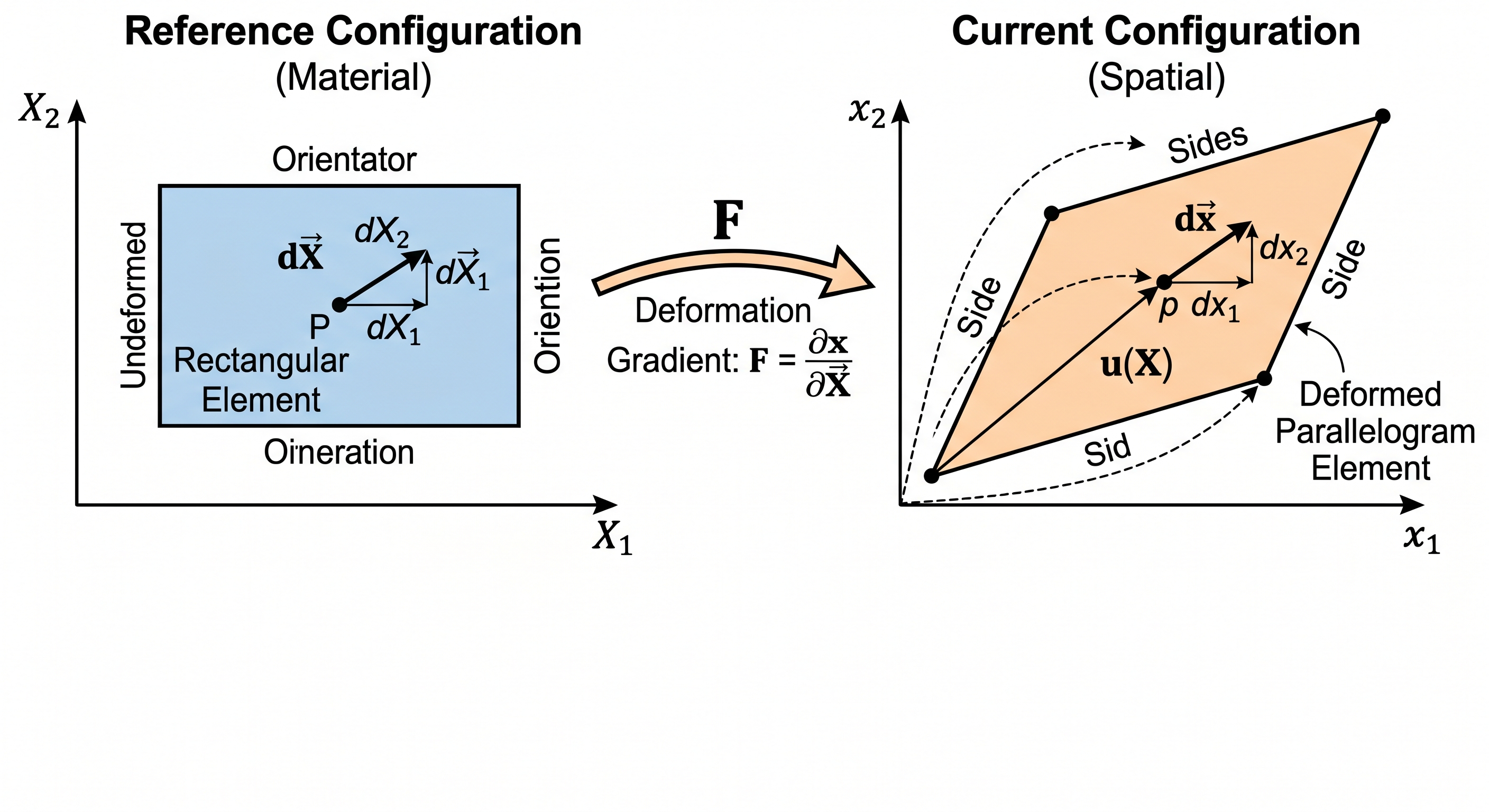
![]()
The deformation map \(\boldsymbol{\chi}\) carries a material point \(\mathbf{X}\) in the reference configuration \(\Omega_0\) to its image \(\mathbf{x} = \boldsymbol{\chi}(\mathbf{X}, t)\) in the current configuration \(\Omega\). The deformation gradient \(\mathbf{F} = \partial\mathbf{x}/\partial\mathbf{X}\) is the local linearisation of this map: it carries the infinitesimal line element \(d\mathbf{X}\) at \(\mathbf{X}\) to \(d\mathbf{x} = \mathbf{F}\,d\mathbf{X}\) at \(\mathbf{x}\). Because \(\mathbf{F}\) has one leg in each configuration (reference-index \(J\), current-index \(i\)), it is a two-point tensor.
Worked Example: Uniaxial Stretch
A uniform stretch: \(x_1 = \lambda_1 X_1, x_2 = \lambda_2 X_2, x_3 = \lambda_3 X_3\).
\[
\mathbf{F} = \begin{pmatrix} \lambda_1 & 0 & 0 \\ 0 & \lambda_2 & 0 \\ 0 & 0 & \lambda_3 \end{pmatrix}, \quad J = \lambda_1\lambda_2\lambda_3.
\]
The principal stretches are the diagonal entries. If \(\lambda_1 > 1\) and \(\lambda_2 = \lambda_3 < 1\) with \(\lambda_1\lambda_2^2 = 1\), the material stretches in one direction and compresses perpendicular to preserve volume (like squeezing a rubber ball in one axis).
Worked Example: Rigid-Body Rotation
A rotation about the \(\mathbf{e}_3\) axis by angle \(\theta\):
\[
\mathbf{F} = \begin{pmatrix} \cos\theta & -\sin\theta & 0 \\ \sin\theta & \cos\theta & 0 \\ 0 & 0 & 1 \end{pmatrix} = \mathbf{R}.
\]
Here, \(\mathbf{F} = \mathbf{R}\) (orthogonal), \(\mathbf{R}^T\mathbf{R} = \mathbf{I}\), and \(J = 1\). The right Cauchy-Green tensor is \(\mathbf{C} = \mathbf{F}^T\mathbf{F} = \mathbf{R}^T\mathbf{R} = \mathbf{I}\). No strain occurs (shape and volume are unchanged); the material simply rotates as a rigid body.
Strain Measures — Extensive Treatment
Motivation: Measuring Change in Length
Consider two neighboring material points separated by an infinitesimal line element \(d\mathbf{X}\) in the reference config. After deformation, they are separated by \(d\mathbf{x} = \mathbf{F} \, d\mathbf{X}\).
The squared lengths are: \[
dS^2 = d\mathbf{X} \cdot d\mathbf{X}, \quad ds^2 = d\mathbf{x} \cdot d\mathbf{x} = (d\mathbf{X})^T \mathbf{F}^T\mathbf{F} \, d\mathbf{X}.
\]
We seek a strain measure that: 1. Vanishes when there is no deformation (\(d\mathbf{x} = d\mathbf{X}\)). 2. Is zero for rigid rotations (where shape is unchanged). 3. Captures the change in length and angle between material line elements.
The key insight is that: \[
ds^2 - dS^2 = d\mathbf{X}^T(\mathbf{F}^T\mathbf{F} - \mathbf{I}) \, d\mathbf{X} = 2 \, d\mathbf{X}^T\mathbf{E} \, d\mathbf{X},
\]
where \(\mathbf{E} = \tfrac{1}{2}(\mathbf{F}^T\mathbf{F} - \mathbf{I})\) is the Green-Lagrange strain tensor.
\[
\mathbf{C} = \mathbf{F}^T\mathbf{F}.
\]
In index notation: \(C_{JK} = F_{iJ}F_{iK}\) (material indices).
Properties: - Symmetric and positive-definite. - Lives in the reference configuration (both indices uppercase). - \(\mathbf{C} = \mathbf{I}\) when there is no deformation.
Physical interpretation: \(\mathbf{C}\) encodes all the deformation information. If we compute \(d\mathbf{X}^T\mathbf{C}\,d\mathbf{X}\), we get \(ds^2\), the squared length in the current config. The components of \(\mathbf{C}\) in a given direction tell us how much that direction has been stretched and rotated.
Green-Lagrange Strain Tensor
\[
\mathbf{E} = \tfrac{1}{2}(\mathbf{C} - \mathbf{I}) = \tfrac{1}{2}(\mathbf{F}^T\mathbf{F} - \mathbf{I}).
\]
Derivation: From \(ds^2 - dS^2 = d\mathbf{X}^T(\mathbf{C} - \mathbf{I}) \, d\mathbf{X}\), we define \(\mathbf{E}\) so that: \[
ds^2 - dS^2 = 2 \, d\mathbf{X}^T\mathbf{E} \, d\mathbf{X}.
\]
The factor of 2 is conventional; it makes the strain “compatible” with the infinitesimal strain (see below).
Properties: - Symmetric, material-configuration tensor. - \(\mathbf{E} = \mathbf{0}\) means \(\mathbf{C} = \mathbf{I}\), i.e., no deformation. - For a rigid rotation, \(\mathbf{F} = \mathbf{R}\), so \(\mathbf{E} = \tfrac{1}{2}(\mathbf{R}^T\mathbf{R} - \mathbf{I}) = \mathbf{0}\) ✓
In terms of displacement: Since \(\mathbf{F} = \mathbf{I} + \nabla_{\mathbf{X}}\mathbf{u}\), \[
\mathbf{E} = \tfrac{1}{2}(\nabla_{\mathbf{X}}\mathbf{u} + \nabla_{\mathbf{X}}\mathbf{u}^T + (\nabla_{\mathbf{X}}\mathbf{u})^T\nabla_{\mathbf{X}}\mathbf{u}).
\]
This is the finite-strain displacement-strain relation. The first two terms (linear in \(\nabla_{\mathbf{X}}\mathbf{u}\)) are the infinitesimal part; the last (quadratic) is the geometric nonlinearity.
\[
\mathbf{b} = \mathbf{F}\mathbf{F}^T.
\]
In index notation: \(b_{ij} = F_{iJ}F_{jJ}\) (spatial indices).
Properties: - Symmetric and positive-definite, spatial-configuration tensor. - \(\mathbf{b} = \mathbf{I}\) when there is no deformation.
Relation to \(\mathbf{C}\): They are not equal, but both encode the stretch information through their eigenvalues. We have: \[
(\mathbf{F}^T\mathbf{F})(\mathbf{F}^{-1}\mathbf{F}^{-T}) = \mathbf{F}^T \mathbf{F},
\] which is different. However, the right and left stretches (to be introduced below) have the same eigenvalues, and so do \(\mathbf{C}\) and \(\mathbf{b}\) (the eigenvalues of \(\mathbf{b}\) are \(\lambda_i^2\)).
Euler-Almansi Strain Tensor
\[
\mathbf{e} = \tfrac{1}{2}(\mathbf{I} - \mathbf{b}^{-1}) = \tfrac{1}{2}(\mathbf{I} - (\mathbf{F}\mathbf{F}^T)^{-1}).
\]
Derivation: Starting from line elements in the spatial config, \(d\mathbf{x}\) and using \(d\mathbf{X} = \mathbf{F}^{-1}d\mathbf{x}\): \[
dS^2 = (d\mathbf{x})^T\mathbf{F}^{-T}\mathbf{F}^{-1}d\mathbf{x}, \quad ds^2 = d\mathbf{x} \cdot d\mathbf{x}.
\]
So \(ds^2 - dS^2 = d\mathbf{x}^T(\mathbf{I} - \mathbf{F}^{-T}\mathbf{F}^{-1})d\mathbf{x} = 2 d\mathbf{x}^T\mathbf{e}\,d\mathbf{x}\), giving \(\mathbf{e} = \tfrac{1}{2}(\mathbf{I} - \mathbf{b}^{-1})\).
Properties: - Symmetric, spatial-configuration tensor. - \(\mathbf{e} = \mathbf{0}\) when \(\mathbf{b} = \mathbf{I}\) (no deformation) ✓ - For rigid rotation, \(\mathbf{e} = \mathbf{0}\) ✓
Relation to Green-Lagrange strain: The pull-back of \(\mathbf{e}\) to the reference config is \(\mathbf{E}\): \[
\mathbf{E} = \mathbf{F}^T\mathbf{e}\mathbf{F}.
\]
Infinitesimal Strain
When deformations are small, \(|\nabla_{\mathbf{X}}\mathbf{u}| \ll 1\), we drop the quadratic terms: \[
\boldsymbol{\varepsilon} = \tfrac{1}{2}(\nabla_{\mathbf{X}}\mathbf{u} + (\nabla_{\mathbf{X}}\mathbf{u})^T) = \operatorname{sym}(\nabla_{\mathbf{X}}\mathbf{u}).
\]
In this limit, \(\mathbf{E} \approx \mathbf{e} \approx \boldsymbol{\varepsilon}\) (all three strain measures converge), and we no longer distinguish reference from spatial coordinates.
Index notation: \(\varepsilon_{ij} = \tfrac{1}{2}\left(\frac{\partial u_i}{\partial X_j} + \frac{\partial u_j}{\partial X_i}\right)\).
Key distinction: \(\mathbf{E}, \mathbf{e}\) are finite-strain measures (finite deformations). \(\boldsymbol{\varepsilon}\) is the small-strain limit. For structures undergoing large deformations (rubber, metals in forming, large-strain plasticity), you must use \(\mathbf{E}\) or \(\mathbf{e}\) and the corresponding constitutive laws (L05, L06). For small deformations (most linear FEA), \(\boldsymbol{\varepsilon}\) and additive decompositions are sufficient (L07–L09).
Two related deformation tensors appear in some literature:
Piola deformation tensor: \(\mathbf{B}_\text{Piola} = \mathbf{C}^{-1} = (\mathbf{F}^T\mathbf{F})^{-1}\). (Note: This is sometimes called the “inverse right Cauchy-Green” and should not be confused with the left Cauchy-Green \(\mathbf{b}\).)
Cauchy deformation tensor: \(\mathbf{c} = \mathbf{b}^{-1} = (\mathbf{F}\mathbf{F}^T)^{-1}\) (spatial). It is the inverse of the Finger tensor.
These are less commonly used in modern courses but appear in classical continuum mechanics texts.
Summary Table
| Right Cauchy-Green |
\(\mathbf{C} = \mathbf{F}^T\mathbf{F}\) |
Reference |
\(\mathbf{I}\) |
| Left Cauchy-Green / Finger |
\(\mathbf{b} = \mathbf{F}\mathbf{F}^T\) |
Current |
\(\mathbf{I}\) |
| Green-Lagrange strain |
\(\mathbf{E} = \tfrac{1}{2}(\mathbf{C} - \mathbf{I})\) |
Reference |
\(\mathbf{0}\) |
| Almansi strain |
\(\mathbf{e} = \tfrac{1}{2}(\mathbf{I} - \mathbf{b}^{-1})\) |
Current |
\(\mathbf{0}\) |
| Infinitesimal strain |
\(\boldsymbol{\varepsilon} = \operatorname{sym}(\nabla_{\mathbf{X}}\mathbf{u})\) |
Either (small-strain) |
\(\mathbf{0}\) |
Stretch and Rotation — Polar Decomposition
Theorem: Unique Polar Decompositions
Theorem. Every invertible deformation gradient \(\mathbf{F}\) can be uniquely decomposed as: \[
\mathbf{F} = \mathbf{R}\mathbf{U} = \mathbf{V}\mathbf{R},
\]
where: - \(\mathbf{R}\) is an orthogonal (rotation) tensor, \(\mathbf{R}^T\mathbf{R} = \mathbf{I}\), \(\det\mathbf{R} = +1\). - \(\mathbf{U}\) is a right stretch tensor (material, symmetric positive-definite). - \(\mathbf{V}\) is a left stretch tensor (spatial, symmetric positive-definite). - \(\mathbf{R}\) is the same in both decompositions; \(\mathbf{V} = \mathbf{R}\mathbf{U}\mathbf{R}^T\) (they are related by a rotation).
Proof sketch: The right Cauchy-Green tensor \(\mathbf{C} = \mathbf{F}^T\mathbf{F}\) is symmetric and positive-definite. It therefore admits a unique symmetric positive-definite square root \(\mathbf{U} = \sqrt{\mathbf{C}}\). Define \(\mathbf{R} = \mathbf{F}\mathbf{U}^{-1}\). Then: \[
\mathbf{R}^T\mathbf{R} = (\mathbf{F}\mathbf{U}^{-1})^T(\mathbf{F}\mathbf{U}^{-1}) = \mathbf{U}^{-1}\mathbf{F}^T\mathbf{F}\mathbf{U}^{-1} = \mathbf{U}^{-1}\mathbf{C}\mathbf{U}^{-1} = \mathbf{U}^{-1}(\mathbf{U}^2)\mathbf{U}^{-1} = \mathbf{I}.
\]
So \(\mathbf{R}\) is orthogonal, \(\det\mathbf{R} = \det\mathbf{F}/\det\mathbf{U} > 0\), thus \(\det\mathbf{R} = +1\). Similarly, \(\mathbf{U} = \mathbf{F}^T\mathbf{F}\) relates to \(\mathbf{V}\) via \(\mathbf{V} = \mathbf{R}\mathbf{U}\mathbf{R}^T\).
The Two Decompositions: Physical Interpretation
Right decomposition (\(\mathbf{F} = \mathbf{R}\mathbf{U}\)):
The material is first stretched by \(\mathbf{U}\) in the reference frame, then rotated by \(\mathbf{R}\) into the current frame.
Physically, imagine a material element: \(\mathbf{U}\) captures the shape change (elongation, shearing) relative to the reference material axes. Then \(\mathbf{R}\) captures the rigid-body rotation of those axes into the current spatial frame.
Left decomposition (\(\mathbf{F} = \mathbf{V}\mathbf{R}\)):
The material is first rotated by \(\mathbf{R}\), then stretched by \(\mathbf{V}\) in the current frame.
Physically, the material first rotates (so the deforming axes align with the current frame), then stretches relative to the current directions.
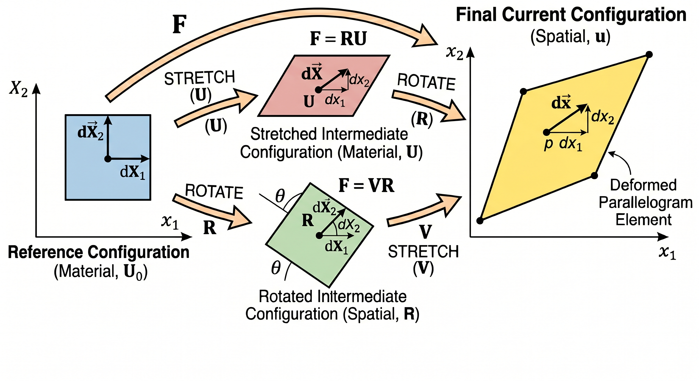
![]()
The two polar decompositions of the deformation gradient \(\mathbf{F}\). Top path (\(\mathbf{F} = \mathbf{R}\mathbf{U}\)): the material is first stretched by \(\mathbf{U}\) along principal directions \(\mathbf{N}_i\) in the reference configuration, then rotated by \(\mathbf{R}\) into its current orientation. Bottom path (\(\mathbf{F} = \mathbf{V}\mathbf{R}\)): the material is first rotated by \(\mathbf{R}\), then stretched by \(\mathbf{V}\) along principal directions \(\mathbf{n}_i = \mathbf{R}\mathbf{N}_i\) in the current configuration. Both paths arrive at the same final state — the decomposition is a matter of where we choose to place the stretch relative to the rotation, not what the material actually does. The two stretches are similar tensors: \(\mathbf{V} = \mathbf{R}\mathbf{U}\mathbf{R}^T\), and they share the eigenvalues \(\lambda_1, \lambda_2, \lambda_3\) — the principal stretches.
Relating the Two Stretches
\[
\mathbf{V} = \mathbf{R}\mathbf{U}\mathbf{R}^T.
\]
This shows that \(\mathbf{U}\) and \(\mathbf{V}\) are similar tensors — they have the same eigenvalues (principal stretches) but eigenvectors rotated by \(\mathbf{R}\).
Relation to Cauchy-Green tensors: \[
\mathbf{C} = \mathbf{F}^T\mathbf{F} = \mathbf{U}^2, \quad \mathbf{b} = \mathbf{F}\mathbf{F}^T = \mathbf{V}^2.
\]
So we compute \(\mathbf{U}\) by taking the symmetric square root of \(\mathbf{C}\), and \(\mathbf{V}\) by taking the symmetric square root of \(\mathbf{b}\).
Principal Stretches
The principal stretches \(\lambda_1, \lambda_2, \lambda_3\) are the eigenvalues of both \(\mathbf{U}\) and \(\mathbf{V}\) (same values, but rotated directions): \[
\lambda_i^2 \text{ are the eigenvalues of } \mathbf{C} \text{ and } \mathbf{b}.
\]
In the principal basis (aligned with the eigenvectors of \(\mathbf{U}\)): \[
\mathbf{U} = \text{diag}(\lambda_1, \lambda_2, \lambda_3), \quad \mathbf{C} = \text{diag}(\lambda_1^2, \lambda_2^2, \lambda_3^2).
\]
Physical interpretation: \(\lambda_i\) is the stretch ratio along the \(i\)-th principal direction. A material fiber initially aligned with the \(i\)-th principal axis is stretched by a factor \(\lambda_i\). For a rigid rotation, \(\lambda_i = 1\) for all \(i\), so \(\mathbf{U} = \mathbf{V} = \mathbf{I}\) and \(\mathbf{F} = \mathbf{R}\).
Worked Example: Simple Shear Polar Decomposition
Consider again \(\mathbf{F} = \begin{pmatrix} 1 & \gamma & 0 \\ 0 & 1 & 0 \\ 0 & 0 & 1 \end{pmatrix}\) (plane shear by \(\gamma\)).
\[
\mathbf{C} = \mathbf{F}^T\mathbf{F} = \begin{pmatrix} 1 & \gamma & 0 \\ \gamma & 1 + \gamma^2 & 0 \\ 0 & 0 & 1 \end{pmatrix}.
\]
For small \(\gamma\), the eigenvalues of \(\mathbf{C}\) are approximately \(\lambda_1^2 \approx 1 + \gamma^2, \lambda_2^2 \approx 1, \lambda_3^2 = 1\), giving \(\lambda_1 \approx 1 + \gamma^2/2, \lambda_2 \approx 1, \lambda_3 = 1\). The deformation consists of a small stretch/compression in two directions and a rotation mixing them.
Spectral Decomposition
We can write \(\mathbf{U}\) and \(\mathbf{V}\) in spectral form: \[
\mathbf{U} = \sum_{i=1}^3 \lambda_i \mathbf{N}_i \otimes \mathbf{N}_i, \quad \mathbf{V} = \sum_{i=1}^3 \lambda_i \mathbf{n}_i \otimes \mathbf{n}_i,
\]
where \(\mathbf{N}_i\) are the principal directions in the reference config (eigenvectors of \(\mathbf{C}\)) and \(\mathbf{n}_i\) are the principal directions in the current config (eigenvectors of \(\mathbf{b}\)). The rotation tensor maps them: \[
\mathbf{n}_i = \mathbf{R}\mathbf{N}_i.
\]
Velocity Gradient and Strain Rate — Extensive Treatment
Definition of Velocity and Velocity Gradient
The velocity field is: \[
\mathbf{v}(\mathbf{x}, t) = \dot{\boldsymbol{\varphi}}(\mathbf{X}, t)
\]
(the material time derivative of position).
The velocity gradient is the spatial gradient of velocity: \[
\mathbf{L} = \nabla_{\mathbf{x}}\mathbf{v} = \frac{\partial v_i}{\partial x_j}\mathbf{e}_i \otimes \mathbf{e}_j.
\]
Fundamental relation: By the chain rule, \[
\dot{\mathbf{F}} = \frac{\partial \dot{\mathbf{x}}}{\partial \mathbf{X}} = \frac{\partial \mathbf{v}}{\partial \mathbf{x}} \cdot \frac{\partial \mathbf{x}}{\partial \mathbf{X}} = \mathbf{L} \cdot \mathbf{F}.
\]
Thus: \[
\mathbf{L} = \dot{\mathbf{F}}\mathbf{F}^{-1}.
\]
This is a key identity: \(\mathbf{L}\) is the time derivative of the deformation gradient in the spatial frame.
The velocity gradient decomposes uniquely into symmetric and skew-symmetric parts: \[
\mathbf{L} = \mathbf{D} + \mathbf{W},
\]
where: - Rate of deformation: \(\mathbf{D} = \operatorname{sym}\mathbf{L} = \tfrac{1}{2}(\mathbf{L} + \mathbf{L}^T)\). - Spin (vorticity): \(\mathbf{W} = \operatorname{skew}\mathbf{L} = \tfrac{1}{2}(\mathbf{L} - \mathbf{L}^T)\).
Index notation: \[
D_{ij} = \tfrac{1}{2}\left(\frac{\partial v_i}{\partial x_j} + \frac{\partial v_j}{\partial x_i}\right), \quad W_{ij} = \tfrac{1}{2}\left(\frac{\partial v_i}{\partial x_j} - \frac{\partial v_j}{\partial x_i}\right).
\]
Physical Interpretation of \(\mathbf{D}\) and \(\mathbf{W}\)
Rate of deformation \(\mathbf{D}\): Measures how line elements are stretching and shearing. If we follow a material line element \(d\mathbf{x}(t)\), its rate of change is: \[
\frac{d}{dt}(d\mathbf{x}) = \mathbf{L} \, d\mathbf{x} = (\mathbf{D} + \mathbf{W}) d\mathbf{x}.
\]
The symmetric part \(\mathbf{D}\) causes the length to change (through \(\mathbf{D}:\mathbf{d}\mathbf{x}\otimes d\mathbf{x}\)) and angles to change (shear).
Spin \(\mathbf{W}\): A skew-symmetric tensor, it represents the local rotation rate. The axial vector of \(\mathbf{W}\) is the angular velocity \(\boldsymbol{\omega}\): \[
\mathbf{W} \mathbf{v} = \boldsymbol{\omega} \times \mathbf{v}
\]
(i.e., \(W_{ij}v_j = \varepsilon_{ijk}\omega_k v_j\)). The spin describes how neighboring material elements rotate relative to one another.
Rate of Green-Lagrange Strain
\[
\dot{\mathbf{E}} = \mathbf{F}^T\mathbf{D}\mathbf{F}.
\]
Derivation: Since \(\mathbf{E} = \tfrac{1}{2}(\mathbf{F}^T\mathbf{F} - \mathbf{I})\), \[
\dot{\mathbf{E}} = \tfrac{1}{2}(\dot{\mathbf{F}}^T\mathbf{F} + \mathbf{F}^T\dot{\mathbf{F}}) = \tfrac{1}{2}((\mathbf{L}\mathbf{F})^T\mathbf{F} + \mathbf{F}^T\mathbf{L}\mathbf{F}) = \tfrac{1}{2}(\mathbf{F}^T\mathbf{L}^T\mathbf{F} + \mathbf{F}^T\mathbf{L}\mathbf{F}) = \mathbf{F}^T\operatorname{sym}(\mathbf{L})\mathbf{F} = \mathbf{F}^T\mathbf{D}\mathbf{F}.
\]
Note that only the symmetric part \(\mathbf{D}\) contributes (the spin \(\mathbf{W}\) does not).
Rate of Jacobian
\[
\dot{J} = J \operatorname{tr}\mathbf{D} = J \operatorname{div}_{\mathbf{x}}\mathbf{v}.
\]
Derivation: \(J = \det\mathbf{F}\), so by the chain rule, \[
\dot{J} = \frac{\partial\det\mathbf{F}}{\partial\mathbf{F}}:\dot{\mathbf{F}} = (\text{cof}\mathbf{F}):\dot{\mathbf{F}} = J(\mathbf{F}^{-T}:\dot{\mathbf{F}}) = J\operatorname{tr}(\mathbf{F}^{-T}\dot{\mathbf{F}}) = J\operatorname{tr}(\mathbf{F}^{-1}\mathbf{L}\mathbf{F}) = J\operatorname{tr}\mathbf{L} = J\operatorname{tr}\mathbf{D}.
\]
Since \(\operatorname{tr}\mathbf{L} = \partial v_i/\partial x_i = \operatorname{div}\mathbf{v}\).
Physical meaning: \(\operatorname{div}\mathbf{v} > 0\) means material is expanding (diverging flow field), \(\operatorname{div}\mathbf{v} < 0\) means it is compressing. For an incompressible material, \(\dot{J} = 0 \Rightarrow \operatorname{div}\mathbf{v} = 0\).
Cartesian Components
In Cartesian coordinates with unit basis: \[
L_{ij} = \frac{\partial v_i}{\partial x_j}, \quad D_{ij} = \tfrac{1}{2}\left(\frac{\partial v_i}{\partial x_j} + \frac{\partial v_j}{\partial x_i}\right), \quad W_{ij} = \tfrac{1}{2}\left(\frac{\partial v_i}{\partial x_j} - \frac{\partial v_j}{\partial x_i}\right).
\]
These are commonly used in finite-strain numerical implementations.
Worked Example: Simple Shear Kinematics
Consider the shearing deformation \(x_1 = X_1 + \gamma(t) X_2, x_2 = X_2, x_3 = X_3\) (shear strain increases with time).
Then \(\mathbf{F} = \begin{pmatrix} 1 & \gamma & 0 \\ 0 & 1 & 0 \\ 0 & 0 & 1 \end{pmatrix}\) and the velocity is \(\mathbf{v} = \dot{\mathbf{F}} X_2 \mathbf{e}_1 = \dot{\gamma}X_2\mathbf{e}_1\) at \(\mathbf{x} = (x_1, x_2, x_3)\).
In spatial coords, \(v_1 = \dot{\gamma}x_2, v_2 = 0, v_3 = 0\).
\[
\mathbf{L} = \begin{pmatrix} 0 & \dot{\gamma} & 0 \\ 0 & 0 & 0 \\ 0 & 0 & 0 \end{pmatrix}, \quad \mathbf{D} = \begin{pmatrix} 0 & \dot{\gamma}/2 & 0 \\ \dot{\gamma}/2 & 0 & 0 \\ 0 & 0 & 0 \end{pmatrix}, \quad \mathbf{W} = \begin{pmatrix} 0 & \dot{\gamma}/2 & 0 \\ -\dot{\gamma}/2 & 0 & 0 \\ 0 & 0 & 0 \end{pmatrix}.
\]
The strain rate \(\mathbf{D}\) shows shear straining in the 1-2 plane; the spin \(\mathbf{W}\) represents the rotation of material fibers (the skew part encodes rigid-body rotation of the material element).
Stress Measures — Four Measures and Transformations
Cauchy (True) Stress
The Cauchy stress tensor \(\boldsymbol{\sigma}\) is defined via Cauchy’s theorem: the traction (force per unit current area) on a surface with unit normal \(\mathbf{n}\) in the current configuration is: \[
\mathbf{t} = \boldsymbol{\sigma}\mathbf{n}, \quad \text{or} \quad t_i = \sigma_{ij}n_j.
\]
Properties: - Spatial (current-config) tensor, both indices lowercase. - Symmetric: \(\boldsymbol{\sigma} = \boldsymbol{\sigma}^T\) (from angular momentum balance). - Measured in force per unit current area: if a patch of material in the current config has area \(da\) and normal \(\mathbf{n}\), the total force is \(\mathbf{t} \, da = \boldsymbol{\sigma}\mathbf{n} \, da\).
Sign convention (per course): Positive in tension, negative in compression. (Some texts use opposite signs.)
Physical interpretation: This is the “true” stress you would measure with a load cell in an experiment. As the material deforms, both the internal stress (force distribution) and the reference area change, so \(\boldsymbol{\sigma}\) reflects the actual mechanical state in the deformed geometry.
First Piola-Kirchhoff Stress
The 1st Piola-Kirchhoff stress (or nominal stress) \(\mathbf{P}\) relates traction in the reference configuration. Define: \[
\mathbf{t}_0 = \mathbf{P}\mathbf{N}, \quad \text{or} \quad t_{0i} = P_{iJ}N_J.
\]
where \(\mathbf{N}\) is the unit normal and \(\mathbf{t}_0\) is the traction on a reference-config surface element with area \(dA\).
To derive the relation between \(\mathbf{P}\) and \(\boldsymbol{\sigma}\), use Nanson’s formula: \[
\mathbf{n} \, da = J\mathbf{F}^{-T}\mathbf{N} \, dA.
\]
Consider a reference surface element with traction \(\mathbf{t}_0 dA\) (resulting in force \(\mathbf{t}_0 dA\)). After deformation, this force is still present but distributed over the current surface, so: \[
\mathbf{t}_0 dA = \boldsymbol{\sigma}\mathbf{n} \, da = \boldsymbol{\sigma}(J\mathbf{F}^{-T}\mathbf{N}) \, dA.
\]
Thus: \[
\mathbf{P}\mathbf{N} = J\boldsymbol{\sigma}\mathbf{F}^{-T}\mathbf{N} \quad \Rightarrow \quad \mathbf{P} = J\boldsymbol{\sigma}\mathbf{F}^{-T}.
\]
Properties: - Two-point tensor: first index spatial (lowercase), second material (uppercase). - Not symmetric in general: \(\mathbf{P} \neq \mathbf{P}^T\) (even though the material is in equilibrium, there is no angular momentum balance in the two-point space). - Measured in force per unit reference area.
Physical interpretation: \(\mathbf{P}\) is useful for Lagrangian formulations because it refers to the known reference configuration. When you specify a displacement boundary condition in FEM, you are working in the reference config; stresses in that frame are naturally expressed via \(\mathbf{P}\).
Second Piola-Kirchhoff Stress
The 2nd Piola-Kirchhoff stress \(\mathbf{S}\) is a pure material-configuration stress defined as: \[
\mathbf{S} = \mathbf{F}^{-1}\mathbf{P} = J\mathbf{F}^{-1}\boldsymbol{\sigma}\mathbf{F}^{-T}.
\]
Properties: - Material (reference) tensor, both indices uppercase. - Symmetric: \(\mathbf{S} = \mathbf{S}^T\).
Why is it symmetric? Unlike \(\mathbf{P}\), the second PK stress lives in the reference configuration alone, where the standard angular momentum argument applies. The pull-back operation \(\mathbf{F}^{-1}(\cdot)\mathbf{F}^{-T}\) preserves symmetry.
Physical interpretation: Although \(\mathbf{S}\) is defined mathematically via \(\mathbf{P}\) and \(\mathbf{F}\), it is the natural “conjugate” stress measure for the Green-Lagrange strain \(\mathbf{E}\) in energy and power expressions (see section 7f below).
Kirchhoff Stress
The Kirchhoff stress is simply a rescaled Cauchy stress: \[
\boldsymbol{\tau} = J\boldsymbol{\sigma}.
\]
Properties: - Spatial (current) tensor, but with a factor of \(J\) that “moves” it toward a material description. - Symmetric (since \(\boldsymbol{\sigma}\) is).
Utility: In incompressible or nearly-incompressible material models, where volume is nearly conserved (\(J \approx 1\)), we have \(\boldsymbol{\tau} \approx \boldsymbol{\sigma}\). The Kirchhoff stress simplifies many energy expressions and is standard in plasticity algorithms (L08).
| Cauchy |
\(\boldsymbol{\sigma}\) |
Current |
Yes |
\(\mathbf{D}\) |
(defined by Cauchy’s theorem) |
| 1st Piola-Kirchhoff |
\(\mathbf{P}\) |
Two-point |
No |
\(\dot{\mathbf{F}}\) |
\(J\boldsymbol{\sigma}\mathbf{F}^{-T}\) |
| 2nd Piola-Kirchhoff |
\(\mathbf{S}\) |
Reference |
Yes |
\(\dot{\mathbf{E}}\) |
\(J\mathbf{F}^{-1}\boldsymbol{\sigma}\mathbf{F}^{-T}\) |
| Kirchhoff |
\(\boldsymbol{\tau}\) |
Current |
Yes |
\(\mathbf{D}\) |
\(J\boldsymbol{\sigma}\) |
Transformation formulas: \[
\mathbf{P} = J\boldsymbol{\sigma}\mathbf{F}^{-T}, \quad \boldsymbol{\sigma} = J^{-1}\mathbf{F}\mathbf{P}, \quad \mathbf{S} = \mathbf{F}^{-1}\mathbf{P} = J\mathbf{F}^{-1}\boldsymbol{\sigma}\mathbf{F}^{-T}.
\]
Worked Example: Uniaxial Loading
Consider the uniaxial tension deformation with \(\lambda_1 = \lambda_2 = \lambda, \lambda_3 = 1/\lambda^2\) (constant volume), giving stretches \(\mathbf{F} = \text{diag}(\lambda, \lambda, 1/\lambda^2)\) and \(J = 1\).
Suppose the material is linearly elastic with modulus \(E\). The Cauchy stress is approximately \(\boldsymbol{\sigma} \approx \begin{pmatrix} E(\lambda - 1/\lambda^4) & 0 & 0 \\ 0 & -0.5E(\lambda - 1/\lambda^4) & 0 \\ 0 & 0 & -0.5E(\lambda - 1/\lambda^4) \end{pmatrix}\) (simplified form for illustration).
The 1st PK becomes \(\mathbf{P} = \boldsymbol{\sigma}\mathbf{F}^{-T} = \begin{pmatrix} E(\lambda - 1/\lambda^4)/\lambda & 0 & 0 \\ 0 & -0.5E(\lambda - 1/\lambda^4)/\lambda & 0 \\ 0 & 0 & -0.5E(\lambda - 1/\lambda^4)\lambda^2 \end{pmatrix}\) (showing the two-point nature: different scalings per component).
Stress-Strain Conjugates and Work Expressions
Power Conjugacy
In the energy balance, the rate of stress power (energy flux) per unit material volume is: \[
P_\text{int} = \int_{\Omega_t} \boldsymbol{\sigma} : \mathbf{D} \, dv = \int_{\Omega_0} \mathbf{P} : \dot{\mathbf{F}} \, dV = \int_{\Omega_0} \mathbf{S} : \dot{\mathbf{E}} \, dV = \int_{\Omega_t} \boldsymbol{\tau} : \mathbf{D} \, dv.
\]
All four expressions are equivalent and equal the rate of internal energy (per unit time). The pairs \((\boldsymbol{\sigma}, \mathbf{D})\), \((\mathbf{P}, \dot{\mathbf{F}})\), \((\mathbf{S}, \dot{\mathbf{E}})\), and \((\boldsymbol{\tau}, \mathbf{D})\) are called work-conjugate pairs.
Derivation (sketch): Start with \(P_\text{int} = \int\boldsymbol{\sigma}:\mathbf{D}\,dv\). Using \(\mathbf{D} = \mathbf{F}^{-T}\dot{\mathbf{E}}\mathbf{F}^{-1}\) (pull-back) and \(dv = J dV\): \[
\int\boldsymbol{\sigma}:\mathbf{D}\,dv = \int\boldsymbol{\sigma}:(\mathbf{F}^{-T}\dot{\mathbf{E}}\mathbf{F}^{-1}) J \, dV.
\]
Rearranging using cyclic permutation of the double contraction: \[
\boldsymbol{\sigma}:(\mathbf{F}^{-T}\dot{\mathbf{E}}\mathbf{F}^{-1}) = (J\mathbf{F}^{-1}\boldsymbol{\sigma}\mathbf{F}^{-T}):\dot{\mathbf{E}} = \mathbf{S}:\dot{\mathbf{E}}.
\]
Thus, \(\int\boldsymbol{\sigma}:\mathbf{D}\,dv = \int\mathbf{S}:\dot{\mathbf{E}} \, dV\) ✓
Implications for Constitutive Laws
In a hyperelastic material, the Helmholtz free energy \(\Psi\) per unit reference volume is a function of the deformation gradient (or strain). The stress is derived from this energy: \[
\mathbf{S} = \rho_0 \frac{\partial\Psi}{\partial\mathbf{E}}, \quad \boldsymbol{\sigma} = J^{-1}\mathbf{F}\mathbf{S}\mathbf{F}^T = J^{-1}\rho_0\mathbf{F}\frac{\partial\Psi}{\partial\mathbf{E}}\mathbf{F}^T.
\]
The choice of which pair to use depends on the formulation: - Lagrangian FEM (material-frame): Use \((\mathbf{S}, \dot{\mathbf{E}})\) or \((\mathbf{P}, \dot{\mathbf{F}})\). - Eulerian FEM (spatial-frame): Use \((\boldsymbol{\sigma}, \mathbf{D})\) or \((\boldsymbol{\tau}, \mathbf{D})\). - Plasticity (usually Lagrangian): Use \((\mathbf{S}, \dot{\mathbf{E}})\) or \((\boldsymbol{\sigma}, \mathbf{D})\) depending on the strain measure.
The equivalence of the power expressions ensures thermodynamic consistency across all formulations.